文章目录
x2可以用x1来表示

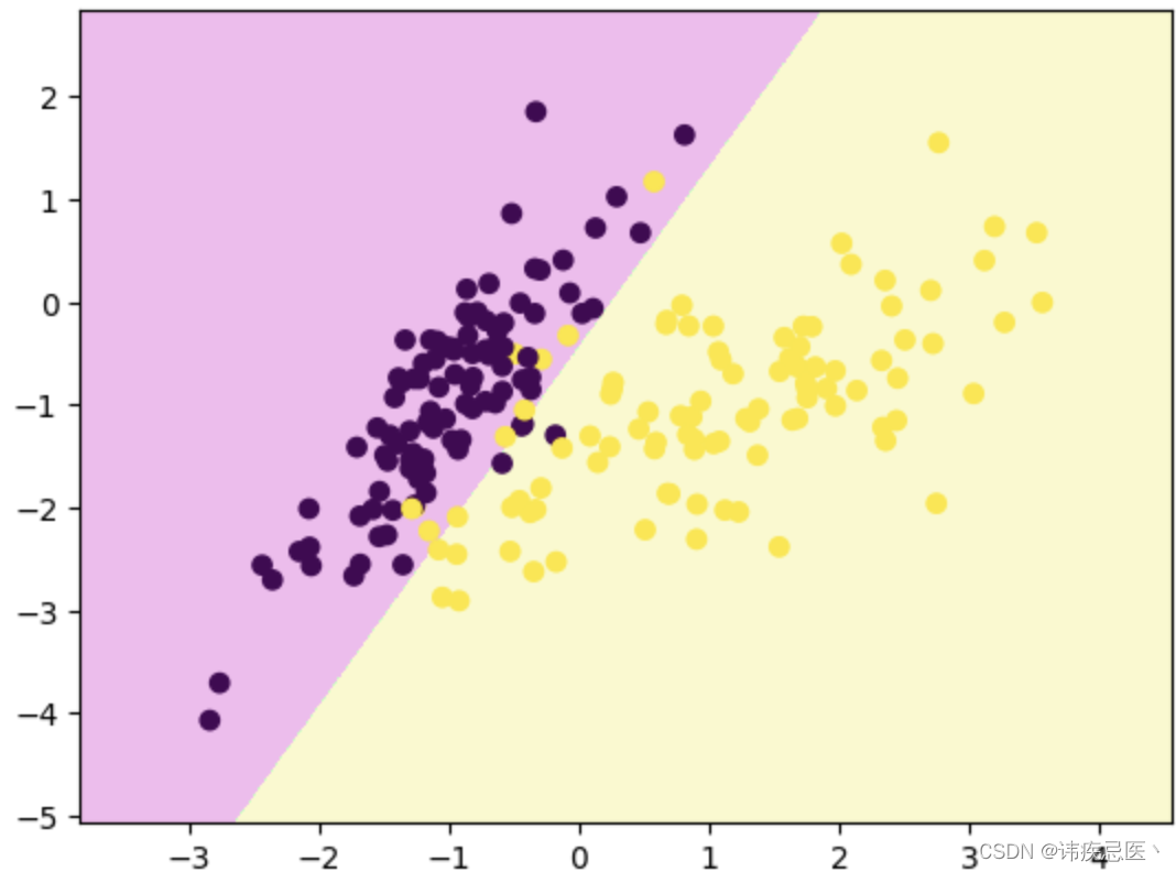
1、线性逻辑回归决策边界
# 逻辑回归
import numpy as np
import matplotlib.pyplot as plt
from sklearn.model_selection import train_test_split
from sklearn.datasets import make_classification
x,y = make_classification(
    n_samples=200,# 样本数
    n_features=2,# 特征数
    n_redundant=0,# 冗余特指数
    n_classes=2,# 类型
    n_clusters_per_class=1,# 族设为1
    random_state=1024
)
x.shape,y.shape

x_train,x_test,y_train,y_test = train_test_split(x,y,train_size=0.7,random_state=1024,stratify=y)
plt.scatter(x_train[:,0],x_train[:,1],c=y_train)

from sklearn.linear_model import LogisticRegression
clf = LogisticRegression()
clf.fit(x_train,y_train)
clf.score(x_test,y_test)
# clf.predict(x_test)

x1 = np.linspace(-4,4,1000)
x2 = (-clf.coef_[0][0] * x1 -clf.intercept_)/clf.coef_[0][1]
plt.scatter(x_train[:,0],x_train[:,1],c=y_train)
plt.scatter(x1,x2)
plt.show()

1.2、使用自定义函数绘制决策边界
很多时候不只是画一条线
def decision_boundary_plot(X, y, clf):
    axis_x1_min, axis_x1_max = X[:,0].min() - 1, X[:,0].max() + 1
    axis_x2_min, axis_x2_max = X[:,1].min() - 1, X[:,1].max() + 1

    x1, x2 = np.meshgrid( np.arange(axis_x1_min,axis_x1_max, 0.01) , np.arange(axis_x2_min,axis_x2_max, 0.01))
    z = clf.predict(np.c_[x1.ravel(),x2.ravel()])
    z = z.reshape(x1.shape)

    from matplotlib.colors import ListedColormap
    custom_cmap = ListedColormap(['#F5B9EF','#BBFFBB','#F9F9CB'])

    plt.contourf(x1, x2, z, cmap=custom_cmap)
    plt.scatter(X[:,0], X[:,1], c=y)
    plt.show()


decision_boundary_plot(x, y ,clf)
1.3、三分类的决策边界
from sklearn import datasets
iris = datasets.load_iris()
x = iris.data[:,:2]
y = iris.target
x_train, x_test, y_train, y_test = train_test_split(x, y, random_state=666)
plt.scatter(x_train[:,0], x_train[:,1], c = y_train)
plt.show()

clf.score(x_test, y_test)
decision_boundary_plot(x, y, clf)

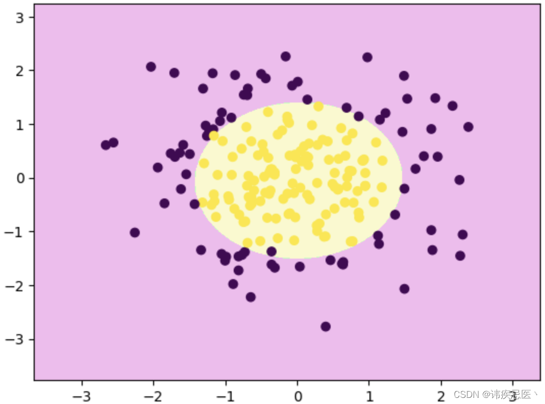
1.4、多项式逻辑回归决策边界
np.random.seed(0)
x = np.random.normal(0, 1, size=(200, 2))
y = np.array((x[:,0]**2+x[:,1]**2)<2, dtype='int')
x_train, x_test, y_train, y_test = train_test_split(x, y, train_size = 0.7, random_state = 233, stratify = y)
plt.scatter(x_train[:,0], x_train[:,1], c = y_train)
plt.show()


from sklearn.pipeline import Pipeline
from sklearn.preprocessing import PolynomialFeatures
from sklearn.preprocessing import StandardScaler
clf_pipe = Pipeline([
        ('poly', PolynomialFeatures(degree=2)),
        ('std_scaler', StandardScaler()),
        ('log_reg', LogisticRegression())
    ])

clf_pipe.fit(x_train, y_train)
decision_boundary_plot(x, y, clf_pipe)
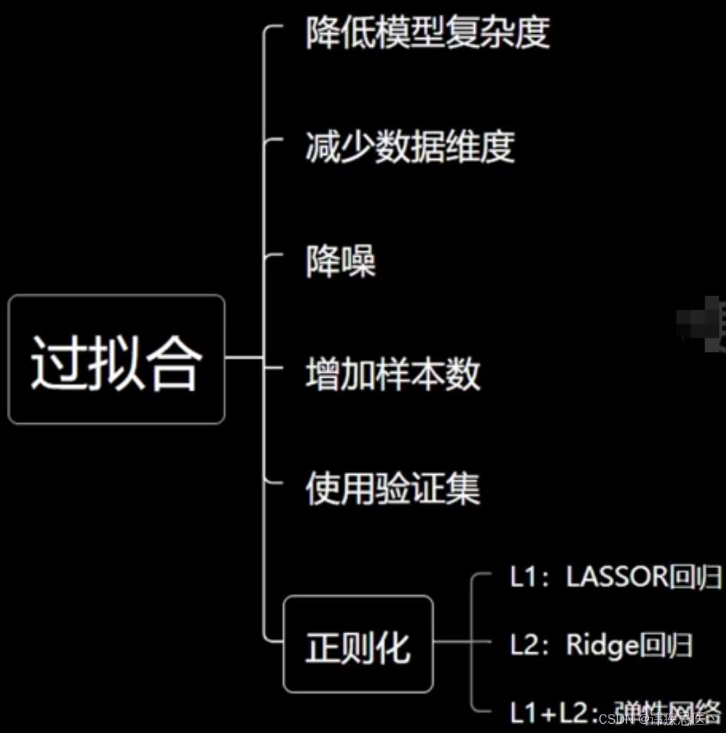
2、过拟合和欠拟合
2.2、欠拟合
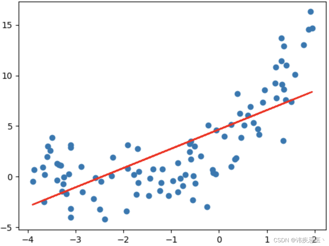
特征维度不足,模型复杂度角度,无法学习到数据背后的规律,使用一元线性回归拟合抛物线数据自然会导致欠拟合
import numpy as np
import matplotlib.pyplot as plt
np.random.seed(233)
x = np.random.uniform(-4, 2, size = (100))
y = x ** 2 + 4 * x + 3 + 2 * np.random.randn(100)

X = x.reshape(-1, 1)

plt.scatter(x,y)
plt.show()

from sklearn.linear_model import LinearRegression
linear_regression = LinearRegression()
linear_regression.fit(X, y)
y_predict = linear_regression.predict(X)
plt.scatter(x, y)
plt.plot(x, y_predict, color = 'red')
plt.show()
2.3、过拟合
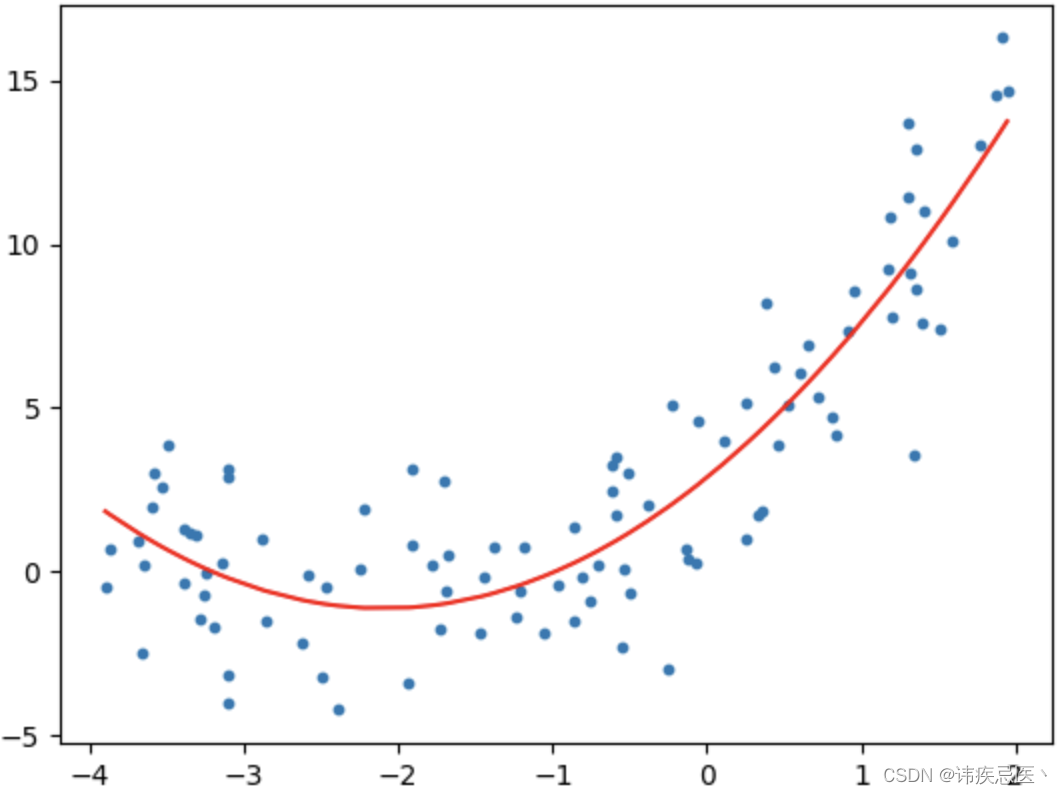
from sklearn.preprocessing import PolynomialFeatures
polynomial_features = PolynomialFeatures(degree=2)
X_poly = polynomial_features.fit_transform(X)
linear_regression = LinearRegression()
linear_regression.fit(X_poly,y)
y_predict = linear_regression.predict(X_poly)
plt.scatter(x,y,s=10)
plt.plot(np.sort(x),y_predict[np.argsort(x)],color='red')
plt.show()

# 另外一种方式
X_new = np.linspace(-5,3,200).reshape(-1,1)
X_new_poly = polynomial_features.fit_transform(X_new)
y_predict = linear_regression.predict(X_new_poly)
plt.scatter(x,y,s=10)
plt.plot(X_new,y_predict,color='red')
plt.show()
print("degree:",2,"score:",linear_regression.score(X_poly,y))
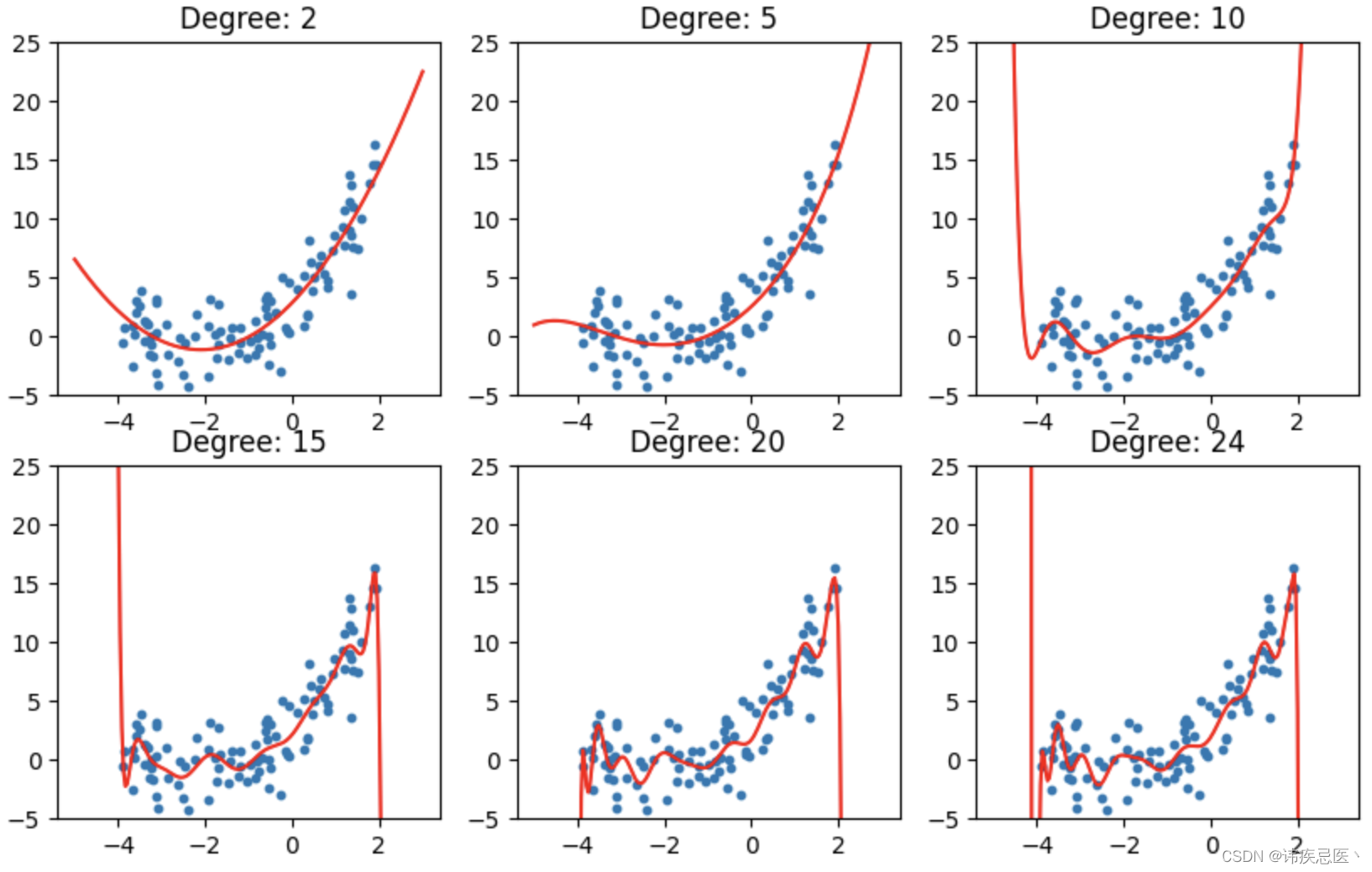
下面三种情况,曲线越来越复杂,与我们的数据相差很远,如果划分了训练集测试机,往往就会在训练集上效果很好,在测试集上效果很差,通俗来讲就是死记了所有习题,但是一考试分数就很低,泛化能力太差。
plt.rcParams["figure.figsize"] = (10, 6)

degrees = [2, 5, 10, 15, 20, 24]
for i, degree in enumerate(degrees):
    polynomial_features = PolynomialFeatures(degree = degree)
    X_poly = polynomial_features.fit_transform(X)

    linear_regression = LinearRegression()
    linear_regression.fit(X_poly, y)

    X_new = np.linspace(-5, 3, 200).reshape(-1, 1)
    X_new_poly = polynomial_features.fit_transform(X_new)
    y_predict = linear_regression.predict(X_new_poly)

    plt.subplot(2, 3, i + 1)
    plt.title("Degree: {0}".format(degree))
    plt.scatter(x, y, s = 10)
    plt.ylim(-5, 25)
    plt.plot(X_new, y_predict, color = 'red')

    print("Degree:", degree, "Score:", linear_regression.score(X_poly, y))

plt.show()
3、学习曲线

从曲线图可以看出来,degree为1的时候误差值比较大,明显是欠拟合状态,为2的时候效果比较好,为5,20的时候明显过拟合状态,训练误差比较小,但是测试误差很大。

from sklearn.metrics import mean_squared_error

plt.rcParams["figure.figsize"] = (12, 8)

degrees = [1, 2, 5, 20]
for i, degree in enumerate(degrees):
    polynomial_features = PolynomialFeatures(degree = degree)

    X_poly_train = polynomial_features.fit_transform(x_train.reshape(-1, 1))
    X_poly_test = polynomial_features.fit_transform(x_test.reshape(-1, 1))

    train_error, test_error = [], []
    for k in range(len(x_train)):
        linear_regression = LinearRegression()
        linear_regression.fit(X_poly_train[:k + 1], y_train[:k + 1])

        y_train_pred = linear_regression.predict(X_poly_train[:k + 1])
        train_error.append(mean_squared_error(y_train[:k + 1], y_train_pred))

        y_test_pred = linear_regression.predict(X_poly_test)
        test_error.append(mean_squared_error(y_test, y_test_pred))

    plt.subplot(2, 2, i + 1)
    plt.title("Degree: {0}".format(degree))
    plt.ylim(-5, 50)
    plt.plot([k + 1 for k in range(len(x_train))], train_error, color = "red", label = 'train')
    plt.plot([k + 1 for k in range(len(x_train))], test_error, color = "blue", label = 'test')
    plt.legend()

plt.show()
4、交叉验证
有没有一种可能就是,模型正好在测试数据集上跑的效果正常,而真实情况是过拟合的,只是没有跑出来,这样的情况下准确性和学习曲线上看似良好,一跑真实数据效果就很差。
解决方法:
多抽几组数据来验证,比如:训练集比作练习题,验证机比作模拟测试,测试机比作考试题。
import numpy as np
from sklearn.model_selection import train_test_split
from sklearn.datasets import load_iris

iris = load_iris()
x = iris.data
y = iris.target

x_train, x_test, y_train, y_test = train_test_split(x, y, train_size = 0.7, random_state = 233, stratify = y)
x_train.shape, x_test.shape, y_train.shape, y_test.shape

from sklearn.model_selection import cross_val_score

neigh = KNeighborsClassifier()
cv_scores = cross_val_score(neigh, x_train, y_train, cv = 5)
print(cv_scores)

best_score = -1
best_n = -1
best_weight = ''
best_p = -1
best_cv_scores = None
for n in range(1, 20):
    for weight in ['uniform', 'distance']:
        for p in range(1, 7):
            neigh = KNeighborsClassifier(
                n_neighbors = n,
                weights = weight,
                p = p
            )
            cv_scores = cross_val_score(neigh, x_train, y_train, cv = 5)
            score = np.mean(cv_scores)
            if score > best_score:
                best_score = score
                best_n = n
                best_weight = weight
                best_p = p
                best_cv_scores = cv_scores

print("n_neighbors:", best_n)
print("weights:", best_weight)
print("p:", best_p)
print("score:", best_score)
print("best_cv_scores:", best_cv_scores)
5、泛化能力
机器学习算法对新鲜事物样本的适应能力,奥卡姆剃刀法则:能简单别复杂,泛化理论:衡量模型复杂度

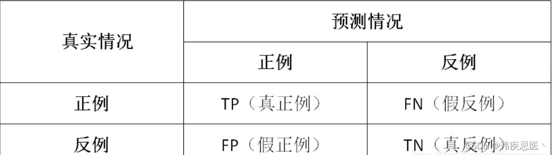
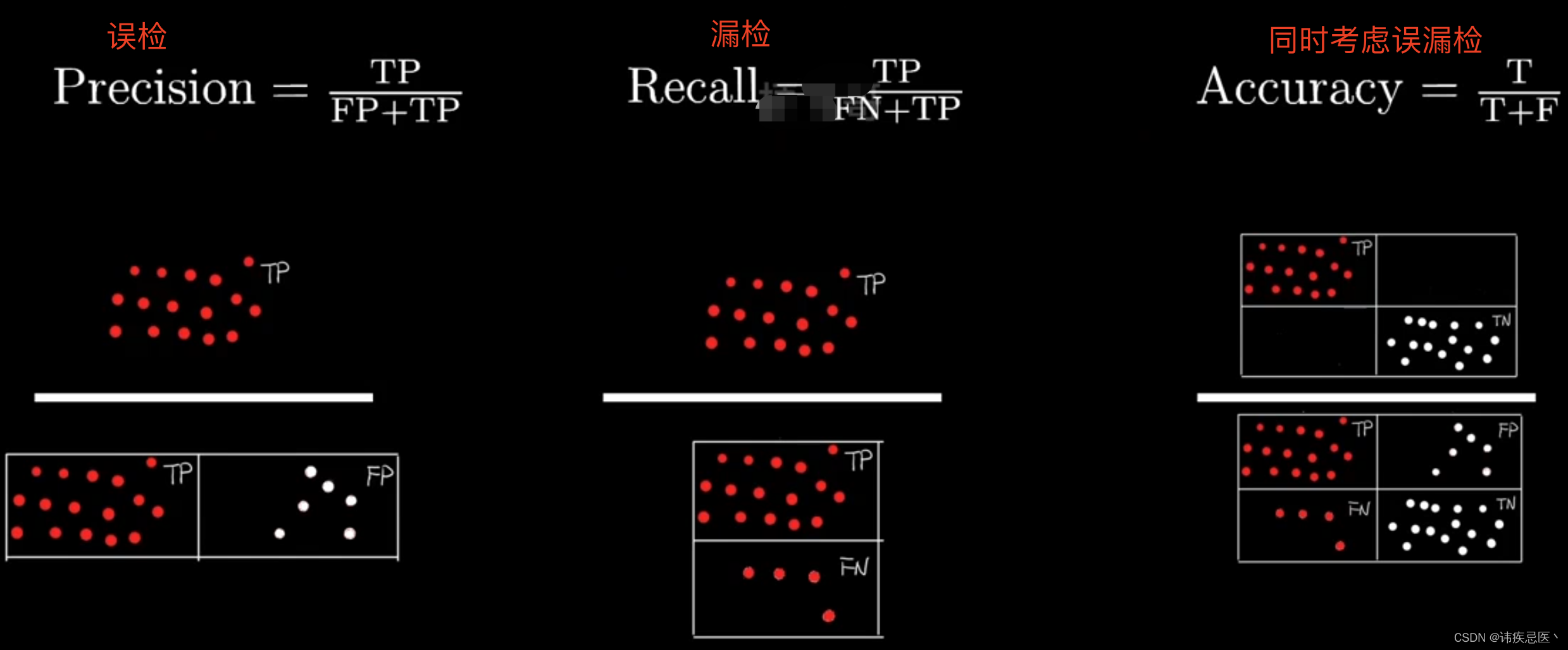
6、混淆矩阵
TP:被模型预测为正类的正样本
TN:被模型预测为负类的负样本
FP:被模型预测为正类的负样本
FN:被模型预测为负类的正样本
TP:被模型预测为好瓜的好瓜(是真正的好瓜,而且也被模型预测为好瓜)
TN:被模型预测为坏瓜的坏瓜(是真正的坏瓜,而且也被模型预测为坏瓜)
FP:被模型预测为好瓜的坏瓜(瓜是真正的坏瓜,但是被模型预测为了好瓜)
FN:被模型预测为坏瓜的好瓜(瓜是真正的好瓜,但是被模型预测为了坏瓜)
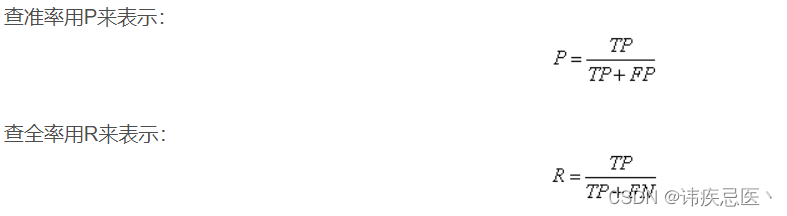
查准率、查全率代表的含义
查准率:模型挑出来的西瓜中有多少比例是好瓜
查全率:所有的好瓜中有多少比例是被模型挑出来的

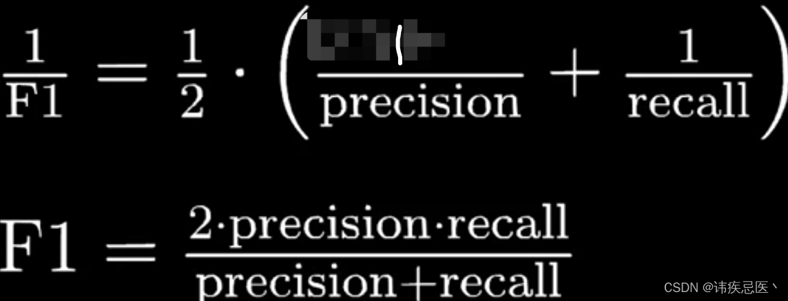
F1 Score
iris = datasets.load_iris()
X = iris.data
y = iris.target.copy()

# 变成二分类
y[y!=0] = 1

from sklearn.model_selection import train_test_split
from sklearn.linear_model import LogisticRegression

X_train, X_test, y_train, y_test = train_test_split(X, y, random_state=666)

logistic_regression = LogisticRegression()
logistic_regression.fit(X_train,y_train)
y_predict = logistic_regression.predict(X_test)

TN = np.sum((y_predict==0)&(y_test==0))
TN

FP = np.sum((y_predict==1)&(y_test==0))
FP

FN = np.sum((y_predict==0)&(y_test==1))
FN

TP = np.sum((y_predict==1)&(y_test==1))
TP

confusion_matrix = np.array([
    [TN, FP],
    [FN, TP]
])

confusion_matrix

precision = TP/ (TP+FP)
precision

recall = TP/(FN+TP)
recall

f1_score = 2*precision*recall /(precision+recall)
f1_score

from sklearn.metrics import confusion_matrix
confusion_matrix(y_test,y_predict)

from sklearn.metrics import precision_score
precision_score(y_test,y_predict)

from sklearn.metrics import recall_score
recall_score(y_test,y_predict)

from sklearn.metrics import f1_score
f1_score(y_test,y_predict)
7、PR曲线和ROC曲线
import numpy as np
import matplotlib.pyplot as plt
from sklearn import datasets

iris = datasets.load_iris()
X = iris.data
y = iris.target.copy()

# 转化为二分类问题
y[y!=0] = 1

from sklearn.model_selection import train_test_split
from sklearn.linear_model import LogisticRegression

X_train, X_test, y_train, y_test = train_test_split(X, y, random_state=666)

logistic_regression = LogisticRegression()
logistic_regression.fit(X_train,y_train)
y_predict = logistic_regression.predict(X_test)
y_predict

decision_scores = logistic_regression.decision_function(X_test)
decision_scores

from sklearn.metrics import precision_score
from sklearn.metrics import recall_score

precision_scores = []
recall_scores = []
thresholds = np.sort(decision_scores)
for threshold in thresholds:
    y_predict = np.array(decision_scores>=threshold,dtype='int')
    precision = precision_score(y_test,y_predict)
    recall = recall_score(y_test,y_predict)
    precision_scores.append(precision)
    recall_scores.append(recall)

plt.plot(thresholds, precision_scores, color='r',label="precision")
plt.plot(thresholds, recall_scores, color='b',label="recall")
plt.legend()
plt.show()

plt.plot(recall_scores,precision_scores)
plt.xlabel("Recall")
plt.ylabel("Precision")
plt.show()
sklearn中实现
# sklearn中
from sklearn.metrics import precision_recall_curve

precision_scores, recall_scores,thresholds =  precision_recall_curve(y_test,decision_scores)

plt.plot(thresholds, precision_scores[:-1], color='r',label="precision")
plt.plot(thresholds, recall_scores[:-1], color='b',label="recall")
plt.legend()
plt.show()

plt.plot(recall_scores,precision_scores)
plt.xlabel("Recall")
plt.ylabel("Precision")
plt.show()


# ROC曲线
from sklearn.metrics import roc_curve

fpr, tpr, thresholds = roc_curve(y_test,decision_scores)
plt.plot(fpr,tpr)
plt.xlabel("FPR")
plt.ylabel("TPR")
plt.show()

# AUC
from sklearn.metrics import roc_auc_score

auc = roc_auc_score(y_test,decision_scores)
auc