基于主成分分析的机器学习分类代码

前言

本文内容主要实现基于主成分分析的数据降维和四种经典的机器学习分类算法，包括：支持向量机、随机森林、XGBoost分类器、scikit-learn的梯度提升分类器和Histogram-based Gradient Boosting分类器

1.数据准备

import pickle
import pandas as pd
import numpy as np


# 先进行文件数据检查，由于本文采用的数据是影像数据转换的结果，因此不需要考虑Null值检查与剔除直接采用pandas读取数据
data_path = r'D:\RS_train_auto_select_fzwb.pickle'
df = pd.read_pickle(data_path)
print(df.head(5))
#提取数据与标签
# 查看单张图像特征
df['feature'].shape
df['feature'].dtype
df_to_arry = np.asarray(df['feature'])[0]
print(df_to_arry.shape)
print(df_to_arry)
# 获取对应特征标签
label = np.asarray(df['label_gt'][0])
label_reshape = label[:,np.newaxis]
print(label_reshape.shape)
# 将数据与标签进行拼接
data = np.hstack((df_to_arry,label_reshape))
data.shape
# 将数据转换为数据框并设置列名称
data_list = ['red','gre','blu','x','y','mean','Variance','Homogeneity','Contrast','Dissimilarity','Entropy','Second','Correlation','label']
img_feature = pd.DataFrame(data,columns=data_list)
img_feature.head(5)
# 删除'x','y'列
data = img_feature.drop(['x','y'],axis=1)
data.head(5)

使用RobustScaler对数据进行缩放
RobustScaler() 是 scikit-learn（通常简称为 sklearn）库中的一个工具，用于特征缩放。它通过对中位数和四分位距（IQR）进行计算，来缩放特征值，使其具有一个更鲁棒的分布。这特别适用于有很多离群点（outliers）的数据集，因为RobustScaler不像StandardScaler那样对离群点敏感。

from sklearn.preprocessing import RobustScaler
train_data = data
robust_scaler = RobustScaler()
robust_scaler.fit(train_data.drop('label', axis=1))
train_data_columns = train_data.drop('label', axis=1).columns
scaled_data_train = robust_scaler.transform(train_data.drop('label', axis=1))
scaled_train_data = pd.DataFrame(scaled_data_train, columns=train_data_columns)
scaled_train_data['label'] = train_data['label'].values
data.head(5)

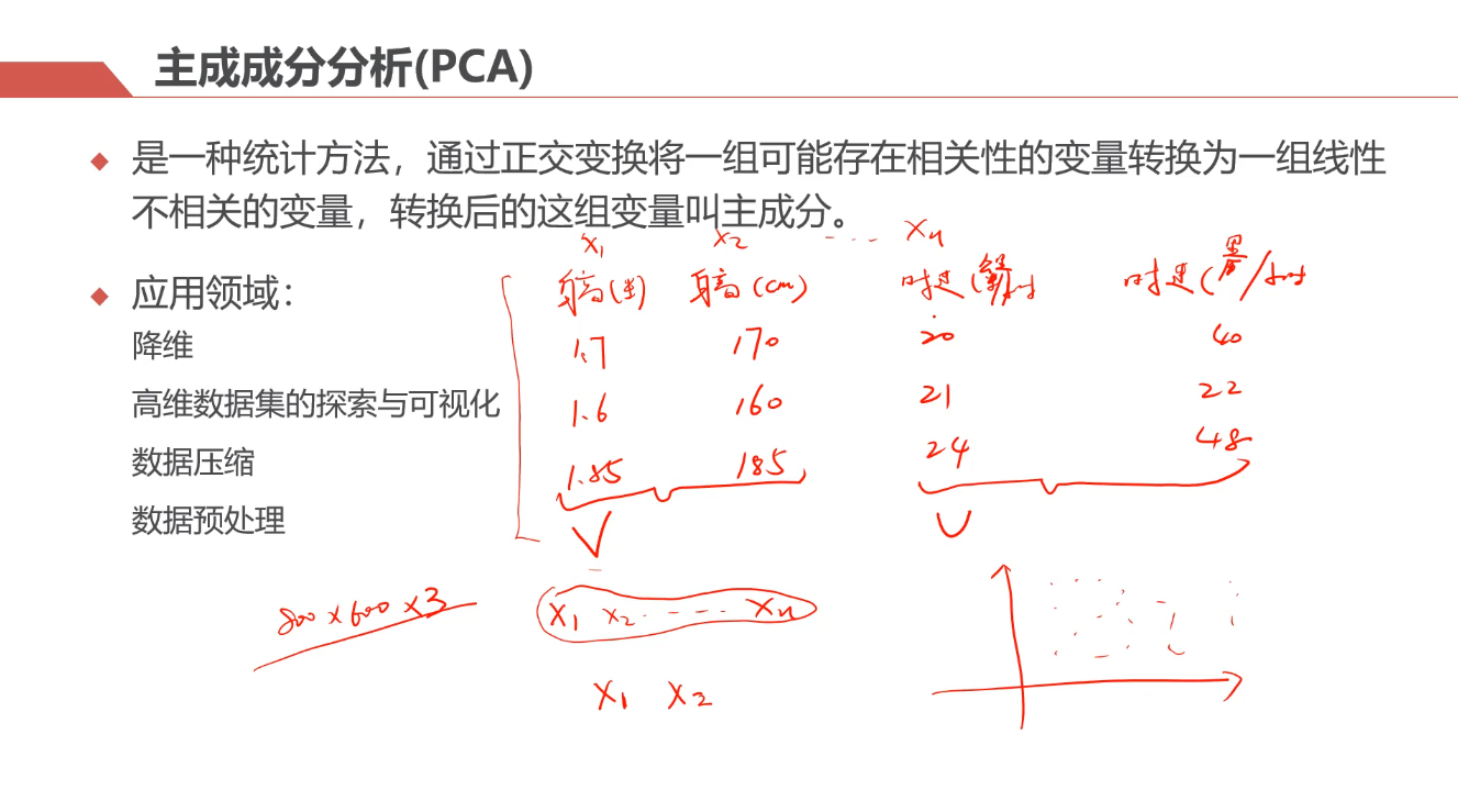
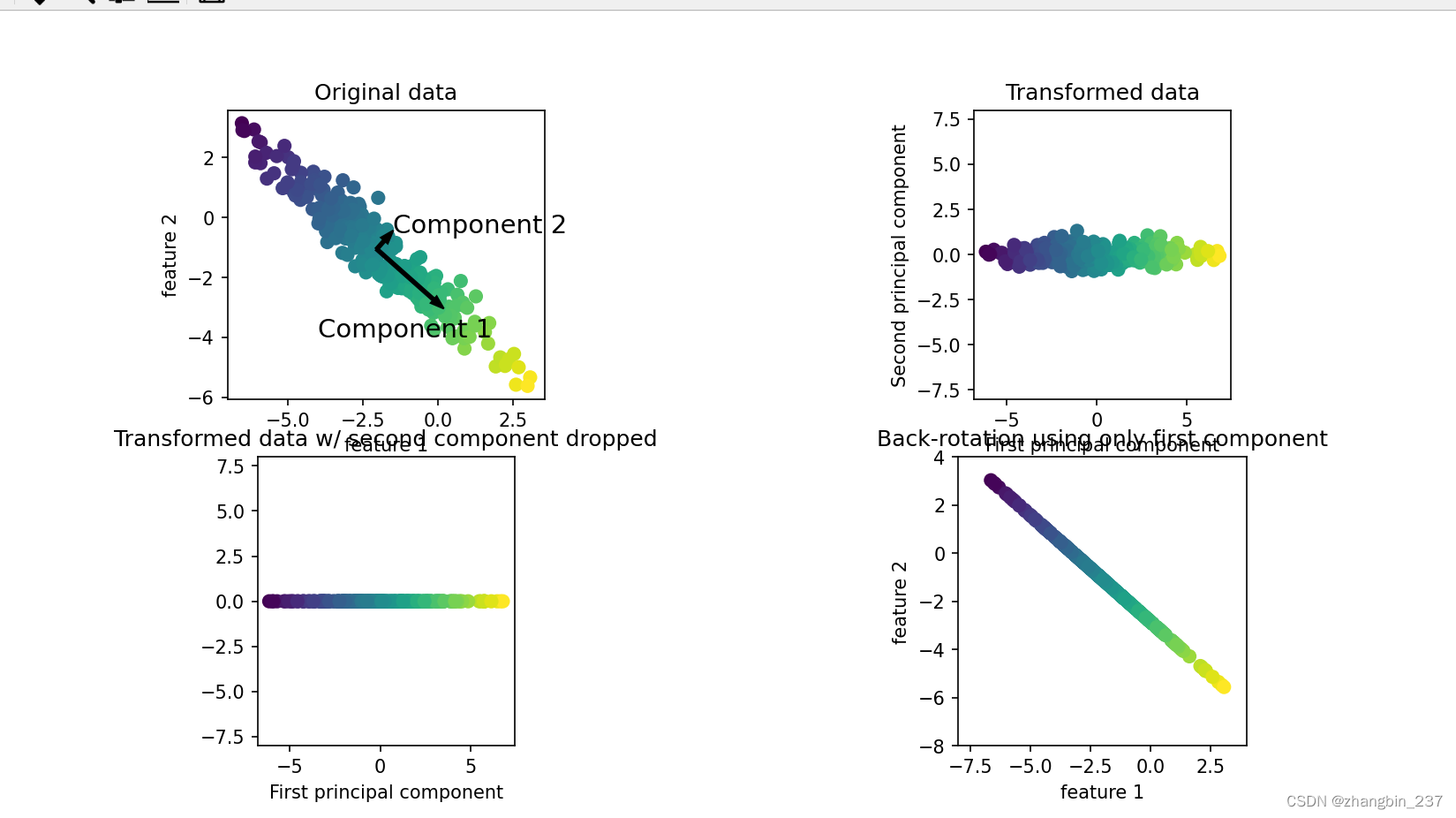
PCA数据降维
pca.explained_variance_ratio_ 是主成分分析（PCA）在 Python 的 scikit-learn 库中返回的一个属性。PCA 是一种用于降低数据维度的统计方法，它可以通过正交变换将原始特征空间中的线性相关变量转换为新的线性无关变量，称为主成分。

explained_variance_ratio_ 属性给出了每个主成分解释的方差的比例。方差是度量数据集中数据点分散程度的一种方式，而解释方差比例则告诉我们每个主成分在解释原始数据集中的方差方面有多重要。

from sklearn.decomposition import PCA
import pandas as pd
import matplotlib.pyplot as plt
# 基于解释方差的寻找最佳组件数量的函数，分析最佳的主成分数量
def find_optimal_components(data, threshold=0.95):
    pca = PCA()
    pca.fit(data)
    # 主成分方差
    explained_variance = pca.explained_variance_ratio_
    cumulative_variance = explained_variance.cumsum()
    # 小于该方差的主成分分量数量
    num_components = len(cumulative_variance[cumulative_variance <= threshold])
    plt.figure(figsize=(10, 6))
    plt.plot(range(1, len(explained_variance) + 1), cumulative_variance, marker='o', linestyle='--')
    plt.title('Cumulative Explained Variance')
    plt.xlabel('Number of Components')
    plt.ylabel('Cumulative Explained Variance')
    plt.axhline(y=threshold, color='r', linestyle='--', label=f'Threshold ({threshold * 100}%)')
    plt.legend()
    plt.show()
    
    return num_components
# Extract target variable 'label'
# 标签
y_tree = scaled_train_df_tree['label']
# 标签中存在异常值15
y_tree[y_tree ==15] = 0
# print(np.unique(y_tree))
# 移除 'label' 列
X = scaled_train_data.drop(['label'], axis=1)
# 寻找最佳的主成分数量
num_components = find_optimal_components(X)
print("最佳特征数量",num_components_tree)
pca = PCA(n_components=num_components)
# 应用主成分分析进行特征统计
pca_train = pca.fit_transform(X)
# 将主成分数据转换为数据框，列为主成分特征，并添加类别列
pca_train = pd.DataFrame(data=pca_train, columns=[f'PC{i}' for i in range(1, num_components + 1)])
pca_train['label'] = y_tree.reset_index(drop=True)
# 查看主成分数据分布
pca_train.describe()

2. 构建训练模型

from sklearn.svm import SVC
from sklearn.ensemble import RandomForestClassifier, GradientBoostingClassifier
from xgboost import XGBClassifier

from sklearn.ensemble import HistGradientBoostingClassifier
# Set a seed for reproducibility
seed = 42

# 初始化模型

svc = SVC(random_state=seed, probability=True)

rf = RandomForestClassifier(random_state=seed)

xgb = XGBClassifier(random_state=seed)

gb = GradientBoostingClassifier(random_state=seed)

hgb = HistGradientBoostingClassifier(random_state=seed)
models = [svc,rf,xgb, gb, hgb]

accuracy_score评价初始化模型

from sklearn.metrics import accuracy_score

def train_test_split_score_classification(model):
    if model in models:
        X = scaled_train_df_tree.drop(['label'], axis=1)
        y = scaled_train_df_tree['label'] 
    # Split into training and testing sets
    X_train, X_test, y_train, y_test = train_test_split(X, y, test_size=0.2, random_state=42)
    
    model.fit(X_train, y_train)
    prediction = model.predict(X_test)
    
    accuracy = accuracy_score(y_test, prediction)
    
    return accuracy

# Use the provided classification models
# 在这里遍历所有模型
models_classification = [svc, rf,  xgb, gb, hgb]

train_test_split_accuracy = []
# 全部模型在训练集上的精度
for model in models_classification:
    print("model:",model)
    train_test_split_accuracy.append(train_test_split_score_classification(model))

3. 精度评价可视化

import scipy.stats as stats
import seaborn as sns
import matplotlib.pyplot as plt

# Create a DataFrame with the scores and sort it
train_test_score_classification = pd.DataFrame(data=train_test_split_accuracy, columns=['Train_Test_Accuracy'])
train_test_score_classification.index = [ 'SVC', 'RF', 'XGB','GB', 'HistGB']

train_test_score_classification = train_test_score_classification.sort_values(by='Train_Test_Accuracy', ascending=False)
train_test_score_classification = train_test_score_classification.round(5)

# Create a bar graph using Seaborn
plt.figure(figsize=(12, 6))
barplot_classification = sns.barplot(x=train_test_score_classification.index, y='Train_Test_Accuracy', data=train_test_score_classification, palette='viridis')

# Add values on the bars
for index, value in enumerate(train_test_score_classification['Train_Test_Accuracy']):
    barplot_classification.text(index, value + 0.001, str(round(value, 5)), ha='center', va='bottom', fontsize=9)
# 可视化
plt.title("Models' Test Score (Accuracy) on Holdout (30%) Set")
plt.xlabel('Models')
plt.ylabel('Accuracy')
plt.xticks(rotation=45)
plt.show()

k折交叉验证

from sklearn.model_selection import train_test_split, StratifiedKFold, cross_val_score
from sklearn.metrics import log_loss
import numpy as np

def train_test_split_score_classification(model, n_splits=5):
    if model in models:
        X = scaled_train_df_tree.drop(['label'], axis=1)
        y = scaled_train_df_tree['label']
 
    
    # Use cross-validation
    cv = StratifiedKFold(n_splits=n_splits, shuffle=True, random_state=42)
    scores = cross_val_score(model, X, y, cv=cv, scoring='neg_log_loss', n_jobs=-1)
        
    # Convert the negative log loss to positive
    loss = -np.mean(scores)
    
    return loss

# Use the provided classification models
models_classification = [svc, rf,  xgb, gb, hgb]

train_test_split_loss = []
cross_val_loss = []

for model in models_classification:
    print("model:",model)
    cross_val_loss.append(train_test_split_score_classification(model))

# Create a DataFrame with the scores and sort it
train_test_score_classification = pd.DataFrame(data={'Cross_Val_Log_Loss': cross_val_loss}, index=['svc', 'rf',  'xgb', 'gb', 'hgb'])

train_test_score_classification = train_test_score_classification.sort_values(by='Cross_Val_Log_Loss', ascending=True)
train_test_score_classification = train_test_score_classification.round(5)

# Create a bar graph using Seaborn
plt.figure(figsize=(12, 6))
barplot_classification = sns.barplot(x=train_test_score_classification.index, y='Cross_Val_Log_Loss', data=train_test_score_classification, palette='viridis')

# Add values on the bars
for index, value in enumerate(train_test_score_classification['Cross_Val_Log_Loss']):
    barplot_classification.text(index, value + 0.001, str(round(value, 5)), ha='center', va='bottom', fontsize=9)

plt.title("Models' Test Score (Log Loss) on Holdout (30%) Set and Cross-Validation")
plt.xlabel('Models')
plt.ylabel('Log Loss')
plt.xticks(rotation=45)
plt.show()

基于optuna的超参数寻优

import optuna
from sklearn.model_selection import train_test_split
from sklearn.metrics import log_loss
from sklearn.ensemble import GradientBoostingClassifier

def objective(trial):
    X_train, X_test, y_train, y_test = train_test_split(scaled_train_df_tree.drop(['label'], axis=1),
                                                        scaled_train_df_tree['label'],
                                                        test_size=0.3,
                                                        random_state=42)


    params = {
        'learning_rate': trial.suggest_float('learning_rate', 0.01, 0.1),
        'n_estimators': trial.suggest_int('n_estimators', 50, 200),
        'max_depth': trial.suggest_int('max_depth', 3, 10),
        'subsample': trial.suggest_float('subsample', 0.6, 1.0),
        'min_samples_split': trial.suggest_int('min_samples_split', 2, 20),
        'min_samples_leaf': trial.suggest_int('min_samples_leaf', 1, 10),
        'max_features': trial.suggest_float('max_features', 0.1, 1.0),
    }

    model = GradientBoostingClassifier(**params, random_state=42)

    model.fit(X_train, y_train)

    prediction_proba = model.predict_proba(X_test)

    loss = log_loss(y_test, prediction_proba)

    return loss
study = optuna.create_study(direction='minimize')
study.optimize(objective, n_trials=50)
print('Best trial:')
trial = study.best_trial
print('Value: {}'.format(trial.value))
print('Params: ')
for key, value in trial.params.items():
    print('{}: {}'.format(key, value))
# 保存模型到文件  
with open(r'D:\GBmodel.pkl', 'wb') as f:  
    pickle.dump(model, f)
# 加载模型  
with open(r'D:\GBmodel.pkl', 'rb') as f:  
    loaded_model = pickle.load(f)  

20240329更新