总结
效应量是荟萃分析的基石。为了进行荟萃分析,我们至少需要估计效应大小及其标准误差。
效应大小的标准误差代表研究对效应估计的精确程度。荟萃分析以更高的精度和更高的权重给出效应量,因为它们可以更好地估计真实效应。
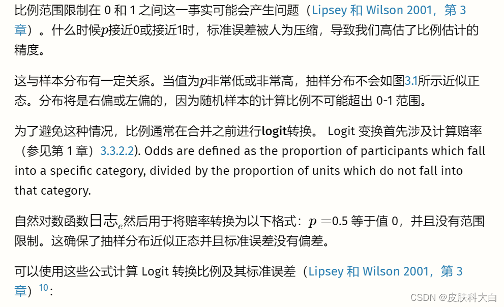
我们可以在荟萃分析中使用多种效应大小。常见的是“单变量”关系度量(例如平均值和比例)、相关性、(标准化)均值差以及风险、优势和发生率比率。
效应大小也可能存在偏差,例如由于测量误差和范围限制。有一些公式可以纠正一些偏差,包括标准化均值差异的小样本偏差、由于不可靠性导致的衰减以及范围限制问题。
其他常见问题是研究报告以不同格式计算效应量所需的数据,以及分析单位问题,当研究贡献不止一种效应量时就会出现这种问题
在第1.1章中,我们将荟萃分析定义为一种总结多项研究定量结果的技术。在荟萃分析中,研究而不是个人成为我们分析的基本单位。
这带来了新的问题。在初步研究中,通常很容易计算汇总统计数据,通过它我们可以描述我们收集的数据。例如,在初步研究中,通常计算连续结果的算术平均值 \(\bar{x}\)和标准差 \(s\) 。
然而,这是可能的,因为在初步研究中通常满足一个基本先决条件:我们知道所有研究对象的结果变量都是以相同的方式测量的。对于荟萃分析,通常不满足此假设。想象一下,我们想要进行一项荟萃分析,我们感兴趣的结果是八年级学生的数学技能。即使我们应用严格的纳入标准(参见第1.4.1章),也可能并非每项研究都使用完全相同的测试来衡量数学技能;有些甚至可能只报告通过或未通过测试的学生比例。这使得几乎不可能直接定量合成结果。
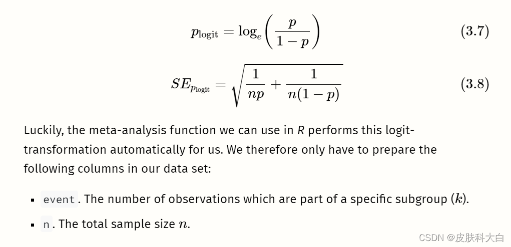
为了进行荟萃分析,我们必须找到一个可以总结所有研究的效应大小。有时,这样的效应量可以直接从出版物中提取;更多时候,我们必须根据研究中报告的其他数据来计算它们。所选的效应量指标可能会对荟萃分析的结果及其可解释性产生重大影响。因此,它们应该满足一些重要标准(Lipsey 和 Wilson 2001;Julian Higgins 等人 2019)。特别是,为荟萃分析选择的效应量测量应该是:
Comparable. It is important that the effect size measure has the same meaning across all studies. Let us take math skills as an example again. It makes no sense to pool differences between experimental and control groups in the number of points achieved on a math test when studies used different tests. Tests may, for example, vary in their level of difficulty, or in the maximum number of points that can be achieved.
Computable. We can only use an effect size metric for our meta-analysis if it is possible to derive its numerical value from the primary study. It must be possible to calculate the effect size for all of the included studies based on their data.
Reliable. Even if it is possible to calculate an effect size for all included studies, we must also be able to pool them statistically. To use some metric in meta-analyses, it must be at least possible to calculate the standard error (see next chapter). It is also important that the format of the effect size is suited for the meta-analytic technique we want to apply, and does not lead to errors or biases in our estimate.
Interpretable. The type of effect size we choose should be appropriate to answer our research question. For example, if we are interested in the strength of an association between two continuous variables, it is conventional to use correlations to express the size of the effect. It is relatively straightforward to interpret the magnitude of a correlation, and many researchers can understand them. In the following chapters, we will learn that it is sometimes not possible to use outcome measures which are both easy to interpret and ideal for our statistical computations. In such cases, it is necessary to transform effect sizes to a format with better mathematical properties before we pool them.
It is very likely that you have already stumbled upon the term “effect size” before. We also used the word here, without paying too much attention to what it precisely stands for. In the next section, we should therefore explore what we actually mean when we talk about an “effect size”.


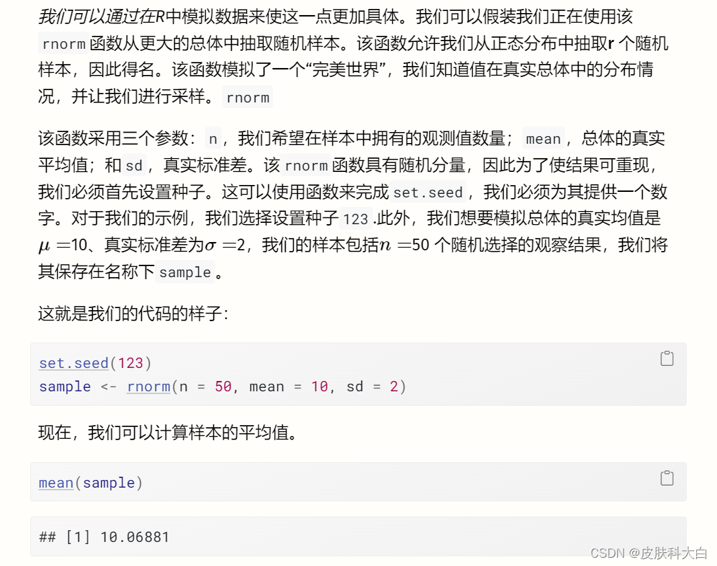
我们看到平均值是 ̄X==10.07,这已经非常接近我们人口的真实值。现在可以通过重复我们在这里所做的事情(随机抽样并计算其平均值)无数次来创建抽样分布。为了为您模拟这个过程,我们执行了之前的步骤 1000 次。
图3.1中的直方图显示了结果。我们可以看到样本的均值非常类似于均值为 10 的正态分布。如果我们抽取更多样本,均值的分布将更加接近正态分布。这一想法在统计学最基本的原则之一——中心极限定理中得到了表达 (Aronow 和 Miller 2019,第 3.2.4 章)。
。
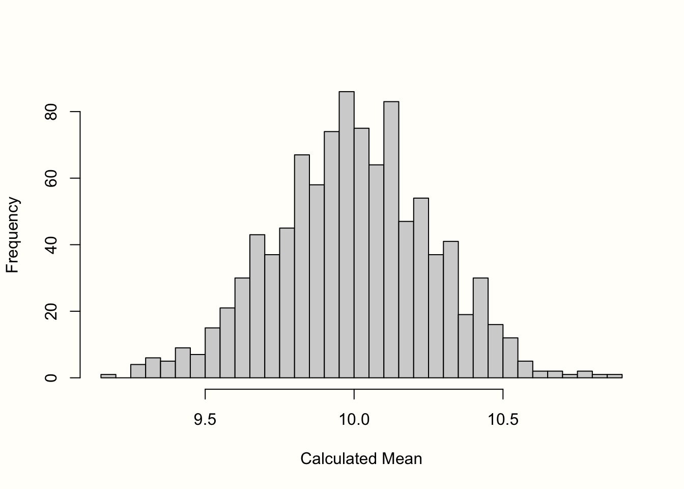
图 3.1:均值的“抽样分布”(1000 个样本)。
标准误差定义为该抽样分布的标准偏差。因此,我们计算了 1000 个模拟均值的标准差,以获得标准误差的近似值。结果是S乙=�乙=0.267。
正如我们之前提到的,我们不能简单地通过模拟真实的抽样分布来计算现实生活中的标准误差。然而,有一些基于统计理论的公式可以让我们计算标准误差的估计值,即使我们仅限于一个观察到的样本(通常是这样)。计算平均值标准误差的公式定义如下: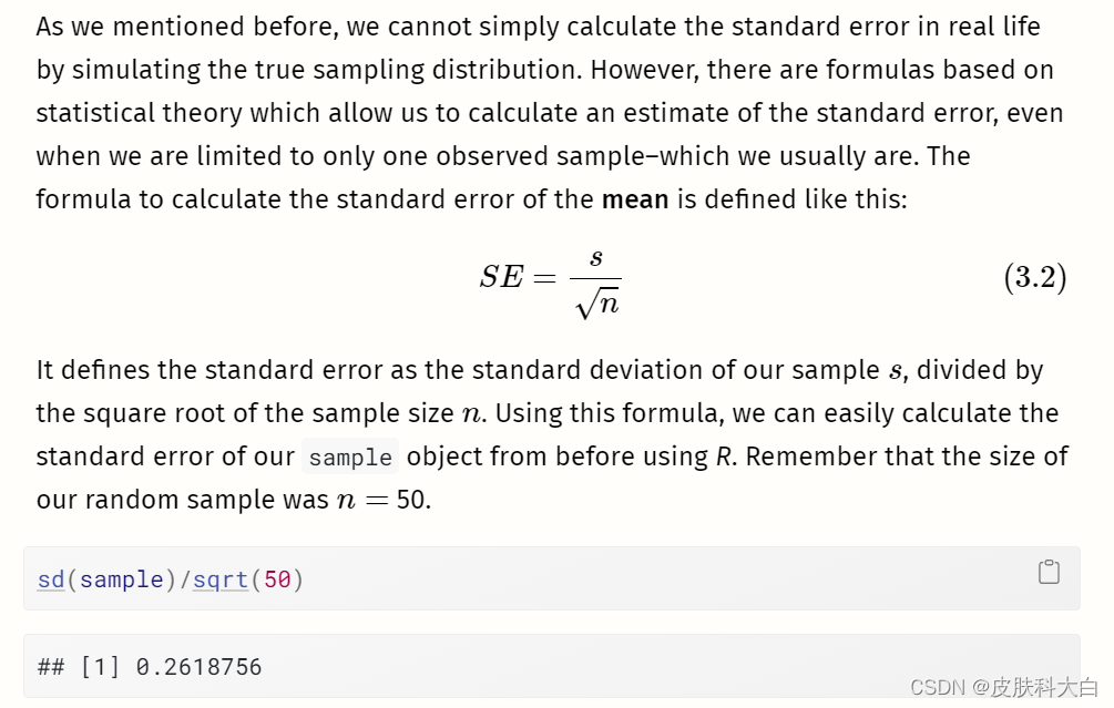

如果我们将该值与我们在抽样分布模拟中发现的值进行比较,我们会发现它们几乎相同。使用该公式,我们可以仅使用我们手头的样本来相当准确地估计标准误差。
在公式 3.2 中,我们可以看到平均值的标准误差取决于研究的样本量。什么时候n�变大,标准误差变小,这意味着研究对真实总体平均值的估计变得更加精确。
为了举例说明这种关系,我们进行了另一次模拟。我们再次使用该rnorm函数,并假设真实总体平均值为μ=�=10 以及那个σ=�=2.但这一次,我们改变了样本量,从n=�=2 至n=�=500. 对于每次模拟,我们使用公式 3.2 计算平均值和标准误差。
## Warning: Using `size` aesthetic for lines was deprecated in ggplot2
## 3.4.0.
## ℹ Please use `linewidth` instead.
## This warning is displayed once every 8 hours.
## Call `lifecycle::last_lifecycle_warnings()` to see where this
## warning was generated.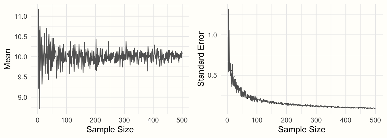
图 3.2:样本平均值和标准误差与样本量的函数关系。
图3.2显示了结果。我们可以看到均值看起来像一个漏斗:随着样本量的增加,均值估计变得越来越精确,并向 10 收敛。这种精度的增加由标准误差表示:随着样本量的增加,标准误差变得越来越小。
我们现在已经探索了进行荟萃分析所需的典型要素:(1)观察到的效应大小或结果测量,以及(2)其精度,以标准误差表示。如果这两类信息可以从已发表的研究中计算出来,通常也可以进行元分析综合(参见第4章)。
在我们的模拟中,我们使用变量的平均值作为示例。重要的是要理解,我们在上面看到的属性也可以在其他结果度量中找到,包括常用的效应量。如果我们计算样本中的平均差而不是平均值,则该平均差将表现出类似形状的抽样分布,并且平均差的标准误差也会随着样本量的增加而减小(假设标准差为保持不变)。同样的情况也成立,例如,(Fisher 的z�变换)相关性。
在以下部分中,我们将介绍荟萃分析中最常用的效应大小和结果测量。这些效应大小指标被如此频繁使用的一个原因是它们满足我们在本章开头定义的两个标准:它们是可靠的和可计算的。
在公式 3.2 中,我们描述了如何计算平均值的标准误差,但该公式只能轻松应用于平均值。其他效应大小和结果测量需要不同的公式来计算标准误差。对于我们在这里介绍的效应大小指标,幸运的是这些公式存在,我们将向您展示所有这些公式。公式的集合也可以在附录中找到。其中一些公式有些复杂,但好消息是我们几乎不需要手动计算标准误差。R中有多种函数可以为我们完成繁重的工作。
在下一节中,我们不仅想提供不同效应大小指标的理论讨论。我们还向您展示了您必须在数据集中准备哪些类型的信息,以便我们稍后使用的R荟萃分析函数可以轻松地为我们计算效应大小。
我们根据效应大小通常出现的研究设计类型对效应大小进行分组:观察设计(例如自然研究或调查)和实验设计(例如对照临床试验)。请注意,这只是一个粗略的分类,而不是严格的规则。我们提出的许多效应量在技术上适用于任何类型的研究设计,只要结果数据的类型适合。

# Set seed of 123 for reproducibility
# and take a random sample (n=50).
set.seed(123)
sample <- rnorm(n = 50, mean = 20, sd = 5)

# Calculate the mean
mean(sample)
## [1] 20.17202# Calculate the standard error
sd(sample)/sqrt(50)## [1] 0.6546889
为了进行均值荟萃分析,我们的数据集至少应包含以下列:
n。研究中的观察次数(样本量)。mean。研究中报告的平均值。sd。研究中报告的变量的标准差。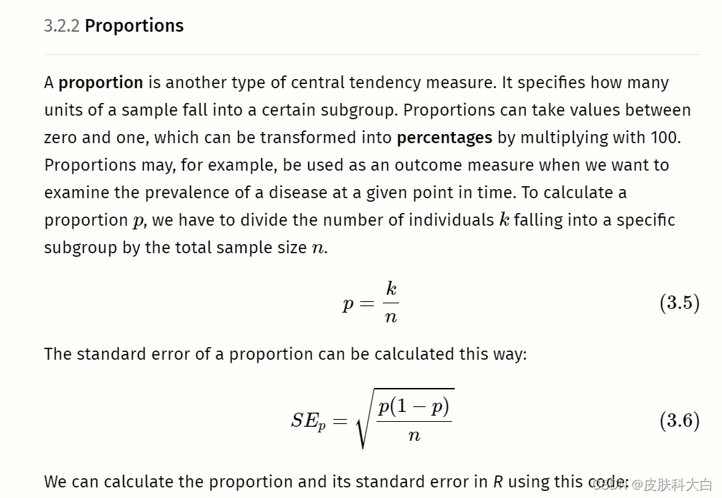
# We define the following values for k and n:
k <- 25
n <- 125

# Calculate the proportion
p <- k/n
p
## [1] 0.2# Calculate the standard error
sqrt((p*(1-p))/n)## [1] 0.03577709


# Simulate two continuous variables x and y
set.seed(12345)
x <- rnorm(20, 50, 10)
y <- rnorm(20, 10, 3)# Calculate the correlation between x and y
r <- cor(x,y)
r
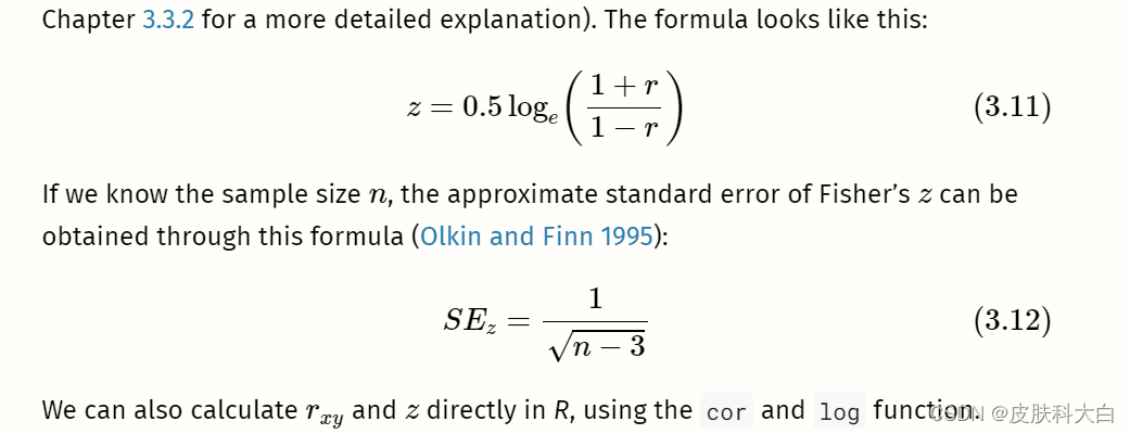
# Calculate Fisher's z
z <- 0.5*log((1+r)/(1-r))
z


# Generate two random variables with different population means
set.seed(123)
x1 <- rnorm(n = 20, mean = 10, sd = 3)
x2 <- rnorm(n = 20, mean = 15, sd = 3)# Calculate values we need for the formulas
s1 <- sd(x1)
s2 <- sd(x2)
n1 <- 20
n2 <- 20
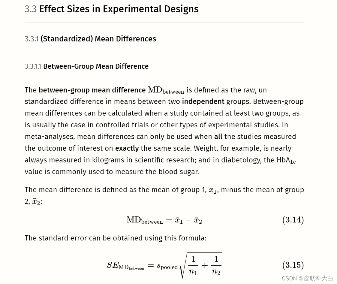
With this data at hand, we can proceed to the core part, in which we calculate the mean difference and its standard error using the formulae we showed before:
# Calculate the mean difference
MD <- mean(x1) - mean(x2)
MD
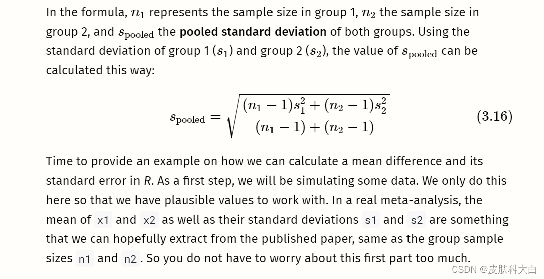
# Calculate s_pooled
s_pooled <- sqrt(
(((n1-1)*s1^2) + ((n2-1)*s2^2))/
((n1-1)+(n2-1))
)# Calculate the standard error
se <- s_pooled*sqrt((1/n1)+(1/n2))
se
通常不需要像我们在这里那样手动进行这些计算。对于均值差异的荟萃分析,我们只需在数据集中准备以下列:
n.e。干预/实验组中的观察数量。mean.e。干预/实验组的平均值。sd.e。干预/实验组的标准差。n.c。对照组中的观察数量。mean.c。对照组的平均值。sd.c。对照组的标准差。
forth13.
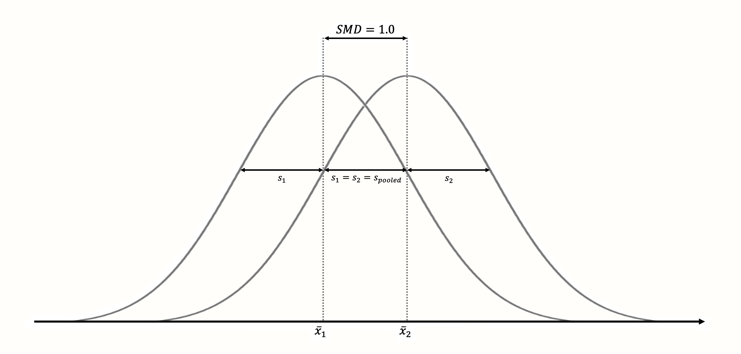
Figure 3.3: Standardized mean difference of 1 (assuming normality, equal standard deviations and equal sample size in both groups).
The standardization makes it much easier to evaluate the magnitude of the mean difference. Standardized mean differences are often interpreted using the conventions by Cohen (1988):
- SMD ≈≈ 0.20: small effect.
- SMD ≈≈ 0.50: moderate effect.
- SMD ≈≈ 0.80: large effect.
Like the convention for Pearson product-moment correlations (Chapter 3.2.3.1), these are rules of thumb at best.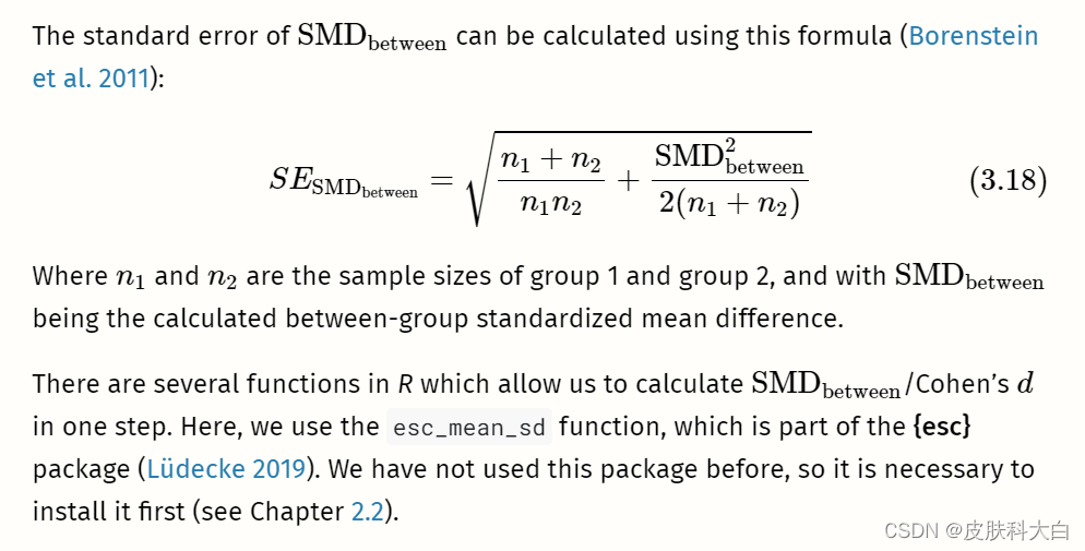
# Load esc package
library(esc)# Define the data we need to calculate SMD/d
# This is just some example data that we made up
grp1m <- 50 # mean of group 1
grp2m <- 60 # mean of group 2
grp1sd <- 10 # sd of group 1
grp2sd <- 10 # sd of group 2
grp1n <- 100 # n of group1
grp2n <- 100 # n of group2# Calculate effect size
esc_mean_sd(grp1m = grp1m, grp2m = grp2m,
grp1sd = grp1sd, grp2sd = grp2sd,
grp1n = grp1n, grp2n = grp2n)
在输出中,有两件事需要提及。首先,我们看到计算出的标准化均值差恰好为 1。这是有道理的,因为我们定义的两个均值之间的差等于(合并的)标准差。
其次,我们看到效应大小是负的。这是因为第 2 组的平均值大于第 1 组的平均值。虽然这在数学上是正确的,但我们有时必须更改计算出的效应大小的符号,以便其他人可以更轻松地解释它们。
想象一下,本例中的数据来自一项研究,测量人们在接受干预(第 1 组)或未接受干预(第 2 组)后每周吸烟的平均数量。在这种情况下,研究结果是积极的,因为干预组的平均吸烟数量较低。因此,将效果大小报告为 1.0 而不是 -1.0 是有意义的,以便其他人可以直观地理解干预具有积极效果。
当一些研究使用的测量值较高意味着更好的结果,而其他研究使用的测量值较低表示更好的结果时,效应大小的符号变得尤为重要。在这种情况下,所有效应大小必须一致地以同一方向编码(例如,我们必须确保在荟萃分析中的所有研究中,较高的效应大小意味着干预组的结果更好)。
通常,小样本校正应用于标准化均值差异,这会产生称为Hedges 的效应大小 G�。我们将在第 3.4.1章中介绍这一更正。
为了对标准化均值差异进行荟萃分析,我们的数据集至少应包含以下列:
n.e。干预/实验组中的观察数量。mean.e。干预/实验组的平均值。sd.e。干预/实验组的标准差。n.c。对照组中的观察数量。mean.c。对照组的平均值。sd.c。对照组的标准差。
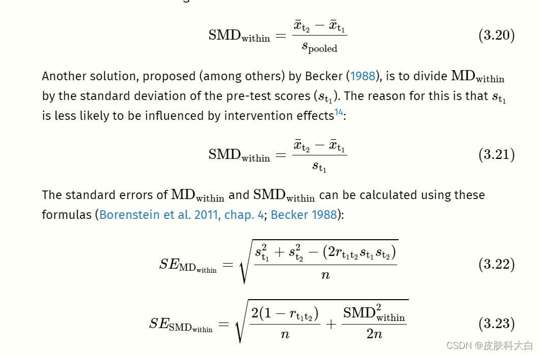
3.3.1.3 Within-Group (Standardized) Mean Difference
Within-group unstandardized or standardized mean differences can be calculated when a difference within one group is examined. This is usually the case when the same group of people is measured at two different time points (e.g. before an intervention and after an intervention).


# Define example data needed for effect size calculation
x1 <- 20 # mean at t1
x2 <- 30 # mean at t2
sd1 <- 13 # sd at t1
n <- 80 # sample size
r <- 0.5 # correlation between t1 and t2# Caclulate the raw mean difference
md_within <- x2 - x1# Calculate the smd:
# Here, we use the standard deviation at t1
# to standardize the mean difference
smd_within <- md_within/sd1
smd_within
# Calculate standard error
se_within <- sqrt(((2*(1-r))/n) +
(smd_within^2/(2*n)))
se_within
Meta-analyses of within-group (standardized) mean differences can only be performed in R using pre-calculated effect sizes (see Chapter 3.5.1). The following columns are required in our data set:
TE: The calculated within-group effect size.seTE: The standard error of the within-group effect size.
The Limits of Standardization
Standardized mean differences are, without a doubt, one of the most frequently used effect sizes metrics in meta-analyses. As we mentioned in Chapter 3.3.1.2, standardization allows us, at least in theory, to compare the strength of an effect observed in different studies; even if these studies did not use the same instruments to measure it.
Standardization, however, is not a “Get Out of Jail Free card”. The size of a particular study’s SMDSMD depends heavily on the variability of its sample (see also Viechtbauer 2007a). Imagine that we conduct two identical studies, use the same instrument to measure our outcome of interest, but that the two studies are conducted in two populations with drastically different variances. In this case, the SMDSMD value of both studies would differ greatly, even if the “raw” mean difference in both studies was identical.
In this case, it is somewhat difficult to argue that the “causal” strength of the effect in one study was much larger or smaller than in the other. As Jacob Cohen (1994) put it in a famous paper: “[t]he effect of A on B for me can hardly depend on whether I’m in a group that varies greatly […] or another that does not vary at all” (p. 1001). This problem, by the way, applies to all commonly used “standardized” effect size metrics in meta-analysis, for example correlations.
In addition, we have also seen that the unit by which to standardize is often less clearly defined than one may think. Various options exist both for between- and within-group SMDSMDs, and it is often hard to disentangle which approach was chosen in a particular study. It is necessary to always be as consistent as possible across studies in terms of how we calculate standardized effect sizes for our meta-analysis. Even so, one should keep in mind that the commensurability of effect sizes can be limited, even if standardization was applied.
Of course, the best solution would be if outcomes were measured on the same scale in all studies, so that raw mean differences could be used. In many research fields, however, we are living far away from such a level of methodological harmony. Thus, unfortunately, standardized effect sizes are often our second best option.
.3.2风险与优势比
3.3.2.1风险比率
正如其名称所示,风险比(也称为相对风险)是两种风险的比率。风险本质上是比例(参见第3.2.2章)。当我们处理二元或二分结果数据时,可以计算它们。
我们使用“风险”一词而不是“比例”,因为这种类型的结果数据经常出现在医学研究中,在医学研究中检查罹患疾病或死亡的风险。此类事件称为事件。想象一下,我们正在进行一项包含治疗组和对照组的对照临床试验。