机器学习 | PCA 主成分分析 (Principal Ccnt Analysis)

通常用于高维数据降维。

擒贼先擒王。

我们为什么要进行降维？

其实机器学习就是模拟一个人的成长过程，小时候有老师教，监督学习 ~

开始的时候会教你这是什么那是什么，就是分类；

当认识的差不多了。就需要自己去想，根据经验判断，就是回归；

长大了，老师不见了，就需要自己去想，无监督学习 ~

没有人告诉你是对是错了，只能靠自己的观察，收集信息，分门别类，就是聚类；

事情越来越多，就需要断舍离，复杂问题简单化，降维。

主 —— 王

成分 —— 空间基

分析 —— 求解、降维

1、核心思想及原理

什么是降维

举个栗子：降维

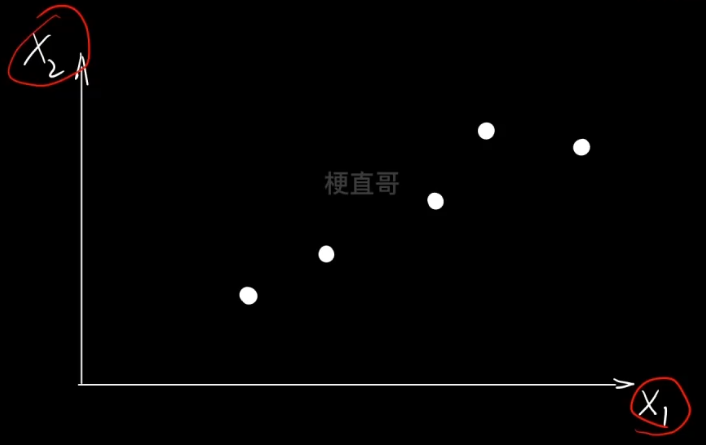
分别投影到x、y轴的分布是不同的。右边显然好一点，正确反映了投影前的位置关系。

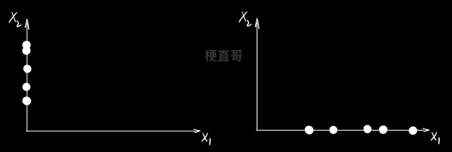
但投影到 x 轴就是最好的嘛？显然不是。

所以降维操作要做的就是找到一条轴，将所有点投影到这条轴上，使得投影后的间距最大。

这就是我们要寻找的主元，就是投影轴。

那用数学语言怎么表示呢？

此时就必须借助线性代数这个工具了，其实线性代数要解决的就是在高维空间中如何描述数据以及这些数据之间的运算。

内积定义和几何解释

数据在高维空间中通常用向量或是矩阵来表示。

高维向量的乘法叫做内积。

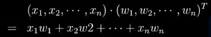
几何含义就是投影。

中学数学其实都是定义在欧几里得空间，而高维向量是定义在内积空间（准希尔伯特空间）。

空间基底

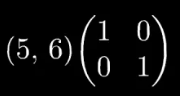
就像空间中的坐标轴一样，可以表达成内积的形式。

下面的结果就是 (5,6) 在以 (1,0),(0,1)为基底的空间中的投影。

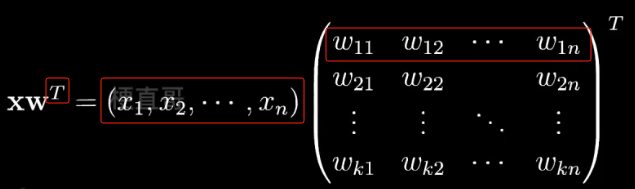
拓展一下，把一个坐标投影到由一组新的基底构成的空间中怎么表示呢？

如下图，其中矩阵 W 其中的每一行都是一个基向量，一共有 k 行，即由 k 个基向量。

数学上我们通常喜欢用一个列向量来表示基向量，

而机器学习中通常使用行向量来表示样本。

姜维的目标就是找到一个最优的特征空间，也就是一个新的基底矩阵，使得维数 k 小于原来的维数 n 。

那怎么才能确保在新的特征空间中数据的分布更好呢，也就是让数据的散度最大？

方差和协方差 —— 衡量数据的散度

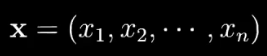
假定现在有n个随机变量，它的向量就是

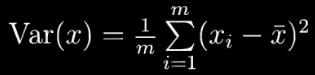
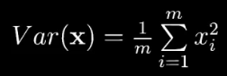
在统计学中，方差就是用来衡量单个随机变量的离散程度

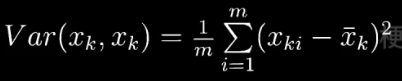
m表示样本的数量，xk i 表示随机变量 xk 的第 i 个观测样本，一共m个。

如果数据预处理均值 = 0，就可以简化成

协方差是用来刻画两个随机变量相似的程度。

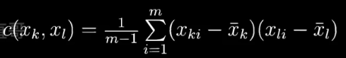
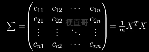
令均值 = 0 就可以简化计算。协方差矩阵就是下面的模样

对角线是方差，其余的均为协方差。

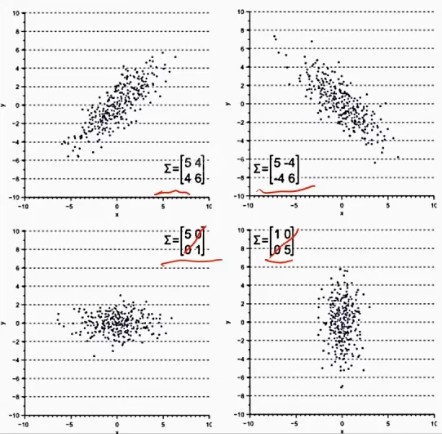
方差的空间几何含义：

在横轴上投影的离散程度就是 x1 的方差。

在纵轴上投影的离散程度就是 x2 的方差。

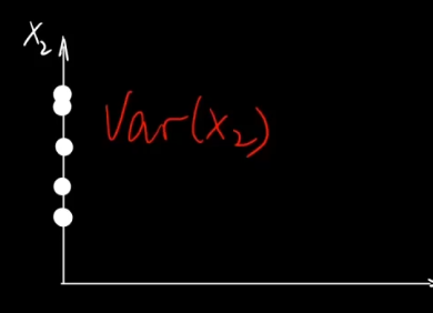
但是都不能准确描述在空间对角线上的离散程度。

协方差矩阵 —— 能够捕捉数据在对角线方向上的离散程度

假设有 m 个 n 维的数据，

降维到数据空间中数据坐标的

方差最大协方差最小的时候最好。

———— 协方差矩阵对角化，找出前面方差大的 k 行做基底。

2、PCA求解算法

协方差矩阵能够捕捉对角倾斜的这种分布。

那怎么找到数据分布的主要方向呢？

特征值和特征向量

特征向量eigenvector

特征值eiger

线性代数中如果一个向量 X 满足：

$AX = \lambda X$

数 $\lambda$ 称为 $A$ 的特征值， $X$ 称为 $A$ 对应于特征值 $\lambda$ 的特征向量。

$A$ 是一个线性变化矩阵，物理上特征值 $\lambda$ 就表示对基向量 $X$ 的缩放程度。

紫色的特征值比较大，它就沿着这个方向伸缩的比较大。

所以我们降维的目的就是为了找到 ——

数据协方差矩阵特征值最大的那些特征向量。

算法步骤

假设我们有 m 条 n 维数据，把它排成一个 mxn 的矩阵

原始数据矩阵化 X 后，零均值化（去掉均值的影响）

求协方差矩阵

求协方差矩阵的特征值和特征向量

按特征值从大到小取特征向量前 k 行组成矩阵 W

即为降维后的数据

注意事项

验证集、测试集执行同样的降维

验证集、测试集执行零均值化操作时，均值须计算于训练集，因为训练集是观测到的数据

保证训练集、测试集独立同分布一致性，否则会出现方差漂移

PCA的主要作用

有效缓解维度灾难

数据降噪效果好，当数据收到噪声影响时，最小特征值对应的特征向量往往和噪声有关

降维后数据特征独立

无法解决过拟合，因为虽然保留了主要信息，但是主要信息主要是针对训练集的，未必是重要信息

3、PCA算法代码实现

import numpy as np
import matplotlib.pyplot as plt

w, b = 1.8, 2.5

np.random.seed(0)
x1 = np.random.rand(100) * 4
noise = np.random.randn(100)
x2 = w * x1 + b + noise

x1.shape, x2.shape

((100,), (100,))

纵向合并：

x = np.vstack([x1, x2]).T
x.shape

(100, 2)

plt.scatter(x[:, 0], x[:, 1])
plt.show()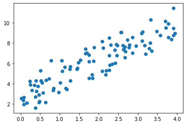

零均值化：

np.mean(x, axis = 0)

array([1.89117536, 6.09644999])

x -= np.mean(x, axis = 0)

plt.scatter(x[:, 0], x[:, 1])
plt.show()

np.mean(x, axis = 0)

array([-1.39888101e-16,  1.49658064e-15])

PCA

from sklearn.decomposition import PCA

pca = PCA(n_components=1)  #主成分个数
pca.fit(x)

PCA

PCA(n_components=1)

pca.components_

array([[0.42746553, 0.90403165]])

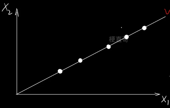
plt.scatter(x[:, 0], x[:, 1], s = 10)
plt.plot(
    np.array([pca.components_[0][0] * -1, pca.components_[0][0]]) * 5,
    np.array([pca.components_[0][1] * -1, pca.components_[0][1]]) * 5,
    c = 'r'
)
plt.show()

x_pca = pca.transform(x)

x_pca.shape

(100, 1)

plt.scatter(x_pca, np.zeros_like(x_pca), s = 10)
plt.show()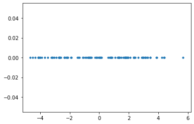

反向映射回原始空间

x_pca_inv = pca.inverse_transform(x_pca)

plt.scatter(x[:, 0], x[:, 1], s = 10)
plt.scatter(x_pca_inv[:, 0], x_pca_inv[:, 1], s = 10, c = 'r')
plt.show()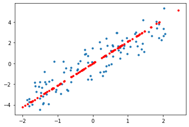

没有完全重合，是因为降维毕竟是有信息损失的，而差异的部分正是投影到轴上的部分。

GPT解释：

PCA降维的过程本质上是将原始数据通过投影到主成分（也可以说是特征向量）所确定的轴上，来实现数据的降维。因此，在进行逆变换时，差异的部分就是未能被完全保留的信息，也就是数据点在垂直于主成分方向的轴上的投影。

具体来说，当我们进行PCA降维时，我们选择了最主要的特征向量作为主成分，这些主成分定义了一个新的坐标系，其中每个主成分都可以看作一个新的轴。当我们进行逆变换时，我们将数据点从这个新的坐标系中映射回原始数据所在的空间，由于数据点在降维过程中丢失了一些信息，因此我们只能重建数据点在主成分方向上的投影，而在垂直于主成分方向上的轴上的投影则无法重建。

因此，差异的部分就是未能被完全保留的信息，也就是数据点在垂直于主成分方向的轴上的投影。这些投影部分被认为是"噪声"或者"误差"，它们在逆变换后会导致重建图像与原始图像之间的差异。

4、降维任务代码实现

4.1、数据集

import numpy as np
import matplotlib.pyplot as plt

from sklearn.datasets import load_digits
digits = load_digits()
x = digits.data
y = digits.target

x.shape, y.shape

((1797, 64), (1797,))

print(digits.DESCR)

.. _digits_dataset:

Optical recognition of handwritten digits dataset
--------------------------------------------------

**Data Set Characteristics:**

    :Number of Instances: 1797
    :Number of Attributes: 64
    :Attribute Information: 8x8 image of integer pixels in the range 0..16.
    :Missing Attribute Values: None
    :Creator: E. Alpaydin (alpaydin '@' boun.edu.tr)
    :Date: July; 1998

This is a copy of the test set of the UCI ML hand-written digits datasets
https://archive.ics.uci.edu/ml/datasets/Optical+Recognition+of+Handwritten+Digits

The data set contains images of hand-written digits: 10 classes where
each class refers to a digit.

Preprocessing programs made available by NIST were used to extract
normalized bitmaps of handwritten digits from a preprinted form. From a
total of 43 people, 30 contributed to the training set and different 13
to the test set. 32x32 bitmaps are divided into nonoverlapping blocks of
4x4 and the number of on pixels are counted in each block. This generates
an input matrix of 8x8 where each element is an integer in the range
0..16. This reduces dimensionality and gives invariance to small
distortions.

For info on NIST preprocessing routines, see M. D. Garris, J. L. Blue, G.
T. Candela, D. L. Dimmick, J. Geist, P. J. Grother, S. A. Janet, and C.
L. Wilson, NIST Form-Based Handprint Recognition System, NISTIR 5469,
1994.

.. topic:: References

  - C. Kaynak (1995) Methods of Combining Multiple Classifiers and Their
    Applications to Handwritten Digit Recognition, MSc Thesis, Institute of
    Graduate Studies in Science and Engineering, Bogazici University.
  - E. Alpaydin, C. Kaynak (1998) Cascading Classifiers, Kybernetika.
  - Ken Tang and Ponnuthurai N. Suganthan and Xi Yao and A. Kai Qin.
    Linear dimensionalityreduction using relevance weighted LDA. School of
    Electrical and Electronic Engineering Nanyang Technological University.
    2005.
  - Claudio Gentile. A New Approximate Maximal Margin Classification
    Algorithm. NIPS. 2000.

from sklearn.model_selection import train_test_split
x_train, x_test, y_train, y_test = train_test_split(x, y, random_state=233)

4.2、PCA降维

from sklearn.decomposition import PCA

pca = PCA()
pca.fit(x_train)

PCA

PCA()

pca.explained_variance_

array([1.81007327e+02, 1.62245915e+02, 1.41965678e+02, 1.00238468e+02,
       6.81939314e+01, 5.82192560e+01, 5.35849636e+01, 4.34003952e+01,
       4.15334270e+01, 3.77412998e+01, 2.95411763e+01, 2.76709665e+01,
       2.14874615e+01, 2.08074313e+01, 1.75469989e+01, 1.69582705e+01,
       1.61421830e+01, 1.51283885e+01, 1.24902934e+01, 1.10196270e+01,
       1.07320199e+01, 9.44840594e+00, 9.09439397e+00, 8.93322578e+00,
       8.46944961e+00, 7.04767976e+00, 6.87546962e+00, 6.31807832e+00,
       5.77351989e+00, 5.18995665e+00, 4.56492303e+00, 4.35442033e+00,
       4.10520804e+00, 3.82441709e+00, 3.72901451e+00, 3.49442464e+00,
       3.17239040e+00, 2.76786099e+00, 2.63864629e+00, 2.57068504e+00,
       2.24762050e+00, 1.85158687e+00, 1.76138992e+00, 1.70038358e+00,
       1.42366072e+00, 1.27843954e+00, 1.13785918e+00, 8.59404411e-01,
       6.72480430e-01, 4.70872656e-01, 3.01051638e-01, 9.86926152e-02,
       6.68544406e-02, 6.52619492e-02, 5.04686299e-02, 1.88299040e-02,
       8.34822998e-03, 1.59088871e-03, 1.50040301e-03, 7.07252921e-04,
       5.25121740e-04, 7.10321039e-31, 7.10321039e-31, 6.79233850e-31])

pca.explained_variance_ratio_

array([1.50332671e-01, 1.34750688e-01, 1.17907268e-01, 8.32514175e-02,
       5.66373528e-02, 4.83530495e-02, 4.45041138e-02, 3.60454873e-02,
       3.44949075e-02, 3.13454184e-02, 2.45349402e-02, 2.29816680e-02,
       1.78460592e-02, 1.72812712e-02, 1.45733726e-02, 1.40844138e-02,
       1.34066257e-02, 1.25646353e-02, 1.03736086e-02, 9.15217073e-03,
       8.91330333e-03, 7.84721880e-03, 7.55319995e-03, 7.41934435e-03,
       7.03416265e-03, 5.85333498e-03, 5.71030867e-03, 5.24737647e-03,
       4.79510238e-03, 4.31043349e-03, 3.79132205e-03, 3.61649248e-03,
       3.40951329e-03, 3.17630697e-03, 3.09707192e-03, 2.90223715e-03,
       2.63477688e-03, 2.29880161e-03, 2.19148445e-03, 2.13504036e-03,
       1.86672439e-03, 1.53780515e-03, 1.46289355e-03, 1.41222573e-03,
       1.18239809e-03, 1.06178702e-03, 9.45030304e-04, 7.13764257e-04,
       5.58517607e-04, 3.91075572e-04, 2.50033507e-04, 8.19675350e-05,
       5.55248606e-05, 5.42022429e-05, 4.19158939e-05, 1.56388684e-05,
       6.93348567e-06, 1.32128656e-06, 1.24613515e-06, 5.87397329e-07,
       4.36131260e-07, 5.89945505e-34, 5.89945505e-34, 5.64126549e-34])

ratio_cum = np.cumsum(pca.explained_variance_ratio_)
ratio_cum

array([0.15033267, 0.28508336, 0.40299063, 0.48624204, 0.5428794 ,
       0.59123245, 0.63573656, 0.67178205, 0.70627696, 0.73762237,
       0.76215731, 0.78513898, 0.80298504, 0.82026631, 0.83483968,
       0.8489241 , 0.86233072, 0.87489536, 0.88526897, 0.89442114,
       0.90333444, 0.91118166, 0.91873486, 0.92615421, 0.93318837,
       0.9390417 , 0.94475201, 0.94999939, 0.95479449, 0.95910492,
       0.96289625, 0.96651274, 0.96992225, 0.97309856, 0.97619563,
       0.97909787, 0.98173264, 0.98403145, 0.98622293, 0.98835797,
       0.9902247 , 0.9917625 , 0.99322539, 0.99463762, 0.99582002,
       0.9968818 , 0.99782684, 0.9985406 , 0.99909912, 0.99949019,
       0.99974023, 0.99982219, 0.99987772, 0.99993192, 0.99997384,
       0.99998948, 0.99999641, 0.99999773, 0.99999898, 0.99999956,
       1.        , 1.        , 1.        , 1.        ])

plt.plot(ratio_cum)
plt.show()

pca = PCA(20)
pca.fit(x_train)

PCA

PCA(n_components=20)

或者

pca = PCA(0.9)
pca.fit(x_train)

PCA

PCA(n_components=0.9)

pca.n_components_

x_train_pca = pca.transform(x_train)
x_test_pca = pca.transform(x_test)

x_train.shape, x_train_pca.shape

((1347, 64), (1347, 21))

4.3、模型训练速度对比

from sklearn.linear_model import LogisticRegression
clf = LogisticRegression(solver = 'saga', tol = 0.001, max_iter = 500, random_state = 233)

%%time
clf.fit(x_train, y_train)
clf.score(x_test, y_test)

CPU times: user 983 ms, sys: 58.2 ms, total: 1.04 s
Wall time: 965 ms

0.9622222222222222

%%time
clf.fit(x_train_pca, y_train)
clf.score(x_test_pca, y_test)

CPU times: user 407 ms, sys: 56.5 ms, total: 463 ms
Wall time: 371 ms

0.9555555555555556

4.4、可视化

pca = PCA(2)
pca.fit(x_train)

PCA

PCA(n_components=2)

x_pca_2d = pca.transform(x_test)

x_pca_2d.shape

(450, 2)

plt.rcParams["figure.figsize"] = (12, 8)
for i, digit in enumerate(y_test):
    plt.scatter(x_pca_2d[i, 0], x_pca_2d[i, 1], color = plt.cm.Dark2(digit), marker = "${0}$".format(digit), s = 60, alpha = 0.5)
plt.show()

5、PCA在数据降噪中的应用

import numpy as np
import matplotlib.pyplot as plt

w, b = 1.8, 2.5

np.random.seed(0)
x1 = np.random.rand(100) * 4
noise = np.random.randn(100)
x2 = w * x1 + b + noise

x = np.vstack([x1, x2]).T
x -= np.mean(x, axis = 0)
x.shape

(100, 2)

plt.scatter(x[:, 0], x[:, 1])
plt.show()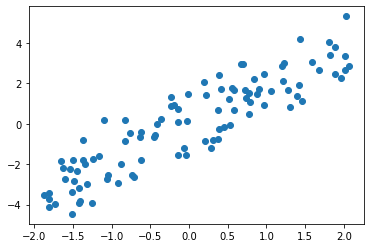

PCA

from sklearn.decomposition import PCA

pca = PCA(n_components=1)
pca.fit(x)

PCA

PCA(n_components=1)

x_pca = pca.transform(x)
x_pca_inv = pca.inverse_transform(x_pca)

plt.scatter(x[:, 0], x[:, 1], s = 10)
plt.scatter(x_pca_inv[:, 0], x_pca_inv[:, 1], s = 10, c = 'r')
plt.show()

图像降噪

from sklearn.datasets import load_digits
digits = load_digits()
x = digits.data
y = digits.target

x.shape, y.shape

((1797, 64), (1797,))

def plot_top20_digits(x):
    for i in range(20):
        plt.subplot(4, 5, i + 1)
        plt.xticks([])
        plt.yticks([])
        plt.imshow(x[i].reshape(8, 8), cmap=plt.cm.gray_r, interpolation="nearest")
    plt.show()

plot_top20_digits(x)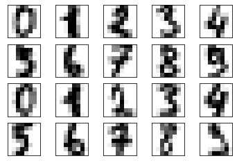

np.random.seed(0)
x_noise = x + np.random.randn(x.shape[0], x.shape[1]) * 3

plot_top20_digits(x_noise)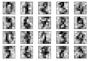

pca = PCA(0.5)
pca.fit(x_noise)
x_noise_pca = pca.transform(x_noise)
x_noise_inv = pca.inverse_transform(x_noise_pca)

plot_top20_digits(x_noise_inv)

6、PCA在人脸识别中的应用

Chapter-13/13-7 PCA在人脸识别中的应用.ipynb · 梗直哥/Machine-Learning - Gitee.com

7、PCA优缺点和适用条件

优点

简单容易计算，易于计算机实现

可以有效减少特征选择工作量，降低算法计算开销

不要求数据正态分布，无参数限制，方差衡量信息，无监督学习，不受样本标签限制

有效去除噪声，使得数据更加容易使用

缺点

非高斯分布情况下，PCA得到的祝愿可能并非最优，ICA（独立主元）也许效果更好

特征值分解的求解方法有一定局限性，如：变换的矩阵必须是方阵

降维后存在信息丢失

主成分解释较原始数据比较模糊

使用条件

变量间强相关数据

数据压缩、预处理

数据降维，噪声去除，去除数据的冗余

高维数据及探索和可视化

参考

Machine-Learning: 《机器学习必修课：经典算法与Python实战》配套代码 - Gitee.com