2024.3.10 机器学习周报

目录

引言

Abstract

文献阅读

1、题目 

2、引言

3、Residual Block的设计

4、ResNet 网络结构

5、创新点

6、实验过程

7、实验结果

Resnet实现

1、ResNet模型搭建（model.py）

2、训练脚本（train.py）

 3、单张图像预测脚本（predict.py）

4、批量图像预测脚本（batch_predict.py）

总结

引言

本周阅读了一篇关于Resnet的文献，文章讨论了在视觉识别任务中训练深度神经网络的困难，并提出了一种残差学习框架来简化这些网络的训练。该框架通过将层次结构重新定义为参考层输入的残差函数来学习，而不是学习无参考函数。该框架通过具有“快捷连接”的前馈神经网络实现，这些连接可以进行恒等映射，而不会增加额外的参数或计算复杂性。并且提供了实证证据表明，这些残差网络更容易优化，并且可以通过增加深度来提高准确性。

Abstract

This week, I read a literature on Resnet, which discussed the difficulties of training deep neural networks in visual recognition tasks and proposed a residual learning framework to simplify the training of these networks. This framework learns by redefining the hierarchical structure as the residual function of the reference layer input, rather than learning without a reference function. This framework is implemented through feedforward neural networks with "fast connections" that can perform identity mapping without adding additional parameters or computational complexity. And empirical evidence is provided to suggest that these residual networks are easier to optimize and can improve accuracy by increasing depth.

文献阅读

1、题目 

Deep Residual Learning for Image Recognition

2、引言

更深的神经网络更难训练。我们提出一个剩余学习框架，以简化培训比所使用的网络深度高得多的网络先前我们明确地将层重新表述为参考层输入的学习残差函数，而不是学习未引用的函数。我们提供了全面的经验证据，表明这些残差网络更容易优化，并且可以从深度显著增加。在ImageNet数据集上，我们评估深度高达152层的残余网——8×比VGG网更深，但仍然具有较低的复性。这些残差网络的集合实现了3.57%的误差在ImageNet测试集上。这一结果在上获得了第一名ILSVRC 2015分类任务。我们还提供了分析在具有100层和1000层的CIFAR-10上。表现的深度至关重要用于许多视觉识别任务。完全由于我们非常深入的表示，我们在COCO对象检测数据集上获得了28%的相对改进。深的残差网是我们提交给ILSVRC的基础和COCO 2015比赛，在那里我们还赢得了第一名介绍了ImageNet检测、ImageNet定位、COCO检测和COCO分割的任务。

3、Residual Block的设计

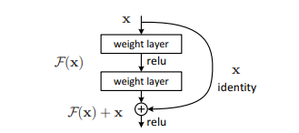
F(x) + x 构成的block称之为Residual Block，即残差块，多个相似的Residual Block串联构成ResNet。一个残差块有2条路径F(x) 和 x，F(x) 路径拟合残差，图中的 ⊕ 为element-wise addition，要求参与运算的F(x) 和 x 的尺寸要相同

左侧残差结构称为 BasicBlock，右侧残差结构称为 Bottleneck，其中第一层的1× 1的卷积核的作用是对特征矩阵进行降维操作，将特征矩阵的深度由256降为64；第三层的1× 1的卷积核是对特征矩阵进行升维操作，将特征矩阵的深度由64升成256。降低特征矩阵的深度主要是为了减少参数的个数。

先降后升为了主分支上输出的特征矩阵和捷径分支上输出的特征矩阵形状相同，以便进行加法操作

4、ResNet 网络结构

ResNet为多个Residual Block的串联，以上能直观看到ResNet-34与34-layer plain net和VGG的对比，以及堆叠不同数量Residual Block得到的不同ResNet

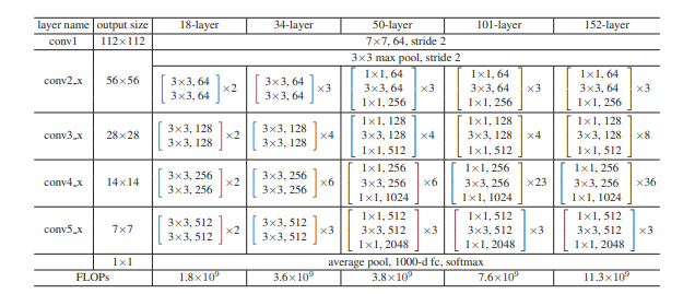
上图是原论文给出的不同深度的ResNet网络结构配置，注意表中的残差结构给出了主分支上卷积核的大小与卷积核个数，表中 残差块×N 表示将该残差结构重复N次

conv3_x, conv4_x, conv5_x所对应的一系列残差结构的第一层残差结构都是虚线残差结构。因为这一系列残差结构的第一层都有调整输入特征矩阵shape的使命（将特征矩阵的高和宽缩减为原来的一半，将深度channel调整成下一层残差结构所需要的channel）

对于ResNet50/101/152，其实conv2_x所对应的一系列残差结构的第一层也是虚线残差结构，因为它需要调整输入特征矩阵的channel。根据表格可知通过3x3的max pool之后输出的特征矩阵shape应该是[56, 56, 64]，但conv2_x所对应的一系列残差结构中的实线残差结构它们期望的输入特征矩阵shape是[56, 56, 256]（因为这样才能保证输入输出特征矩阵shape相同，才能将捷径分支的输出与主分支的输出进行相加）。所以第一层残差结构需要将shape从[56, 56, 64] --> [56, 56, 256]。这里只调整channel维度，高和宽不变（而conv3_x, conv4_x, conv5_x所对应的一系列残差结构的第一层虚线残差结构不仅要调整channel还要将高和宽缩减为原来的一半）

5、创新点

• 提出了residual模块，将深层网络的训练问题转化为逼近残差函数的问题，从而解决了深层网络训练中的退化问题。
• 通过使用快捷连接和元素级相加的方式，实现了残差学习的每几个堆叠层之间的连接，使得网络的训练更加高效。
• 使用Batch Normalization加速训练，丢弃了dropout层，解决梯度消失/梯度爆炸问题
• 在实现方面，采用了批归一化和合适的初始化方法，以及训练策略，进一步提升了网络的性能。

6、实验过程

在包含 1000 个类的 ImageNet 2012 分类数据集上评估方法，这些模型在 128 万张训练图像上进行训练，并在 50k 验证图像上进行评估，我们还获得了测试服务器报告的 100k 测试图像的最终结果，评估前 1 和前 5 的错误率。

对CIFAR-10数据集进行了深入的神经网络有效性分析，该数据集包含10个类别的50k个训练图像和10k个测试图像。使用简单的架构，其中普通/残差架构ResNet网络架构图的形式。实验重点关注极深网络的行为，而不是推动最新的结果。使用了0.0001的权重衰减和0.9的动量，并且模型使用128个mini-batch大小在两个GPU上进行训练，遵循简单的数据增强方案。

7、实验结果

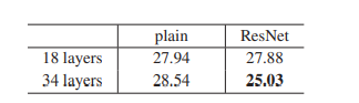
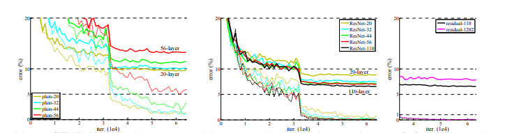
这里的ResNets与它们的普通相比没有额外的参数相对应的人，表明较深的 34 层普通网络比较浅的 18 层普通网络有更高的验证误差。

比较了他们在训练过程中的训练/验证错误。 观察到退化问题，随着网络深度的增加，误差率反而上升，深的普通网络可能指数级的降低的收敛速度，对训练误差的降低产生影响。

结果对比： 1.消除退化问题，并且可推广到验证数据。 2.对比普通网络，34层ResNet将错误降低了3.5，验证了在深度网络上残差学习的有效性。 3.收敛更快，ResNet在早期提供更快的收敛速度。

针对三种shortcuts实验来对比。ImageNet验证的错误率（%，10作物测试）。VGG-16是基于我们的测试。ResNet-50/101/152属于选项B，仅使用投影来增加尺寸。其中，C>B>A，但C牺牲了太多训练时间。考虑采用B方案+深度瓶颈架构加快训练时间。152层的ResNet比VGG16/19 复杂度少得多

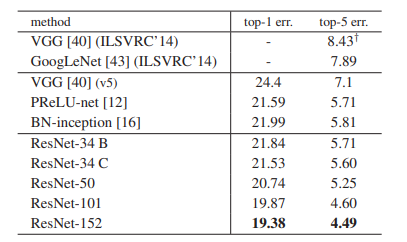
与其他最先进技术的比较。34层已经很好。深度增加后精度也增加，152层top-5的验证误差率达到4.49%。结果优于所有以前的综合模型。其中比赛时ResNet152在测试集上获得了3.57% 的top-5误差。这在2015 ILSVRC获得了第一名

CIFAR-10数据集：训练集：50K；测试集：10K；分10类。 架构：输入32x32的图像，预先减去每一个像素的均值。第一层是3×3卷积层。对于尺寸分别为{32, 16, 8 }的特征图谱分别使用过滤器{16,32,64}，降采样为步长为2的卷积，网络以全局的均值池化终止，10全连通层，softmax。

采用A策略恒等映射，使残差模型跟普通模型有这一模一样的深度、宽度和参数个数。结果网络对数据集依然有很好的效果。

CIFAR10图层响应的标准偏差（std）。响应是每个3×3层的输出，在BN和在非线性之前。顶部：图层显示为原始图层顺序底部：回答按降序排列。展示了残差函数的响应强度，残差函数通常比非残差函数更接近于零，更深的ResNet则具有更小的响应量。当有更多的层时，单个层的ResNets倾向于较少地修改信号

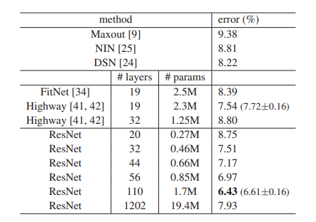
CIFAR-10测试集的分类错误。所有方法都有数据扩充功能。对于ResNet-110，运行了5次并显示最佳（平均值±标准差），1000层没有显示出优化的困难，误差率增加可能是过拟合。

Resnet实现

1、ResNet模型搭建（model.py）

# ResNet整个网络的框架部分
class ResNet(nn.Module):

    def __init__(self,
                 block,   # 残差结构，Basicblock or Bottleneck
                 blocks_num,   # 列表参数，所使用残差结构的数目，如对ResNet-34来说即是[3,4,6,3]
                 num_classes=1000,   # 训练集的分类个数
                 include_top=True):   # 为了能在ResNet网络基础上搭建更加复杂的网络，默认为True
        super(ResNet, self).__init__()
        self.include_top = include_top   # 传入类变量

        self.in_channel = 64   # 通过max pooling之后所得到的特征矩阵的深度

        self.conv1 = nn.Conv2d(3, self.in_channel, kernel_size=7, stride=2,
                               padding=3, bias=False)   # 输入特征矩阵的深度为3（RGB图像），高和宽缩减为原来的一半
        self.bn1 = nn.BatchNorm2d(self.in_channel)
        self.relu = nn.ReLU(inplace=True)

        self.maxpool = nn.MaxPool2d(kernel_size=3, stride=2, padding=1)   # 高和宽缩减为原来的一半

        self.layer1 = self._make_layer(block, 64, blocks_num[0])   # 对应conv2_x
        self.layer2 = self._make_layer(block, 128, blocks_num[1], stride=2)   # 对应conv3_x
        self.layer3 = self._make_layer(block, 256, blocks_num[2], stride=2)   # 对应conv4_x
        self.layer4 = self._make_layer(block, 512, blocks_num[3], stride=2)   # 对应conv5_x

        if self.include_top:   # 默认为True
            # 无论输入特征矩阵的高和宽是多少，通过自适应平均池化下采样层，所得到的高和宽都是1
            self.avgpool = nn.AdaptiveAvgPool2d((1, 1))  # output size = (1, 1)
            self.fc = nn.Linear(512 * block.expansion, num_classes)   # num_classes为分类类别数

        for m in self.modules():   # 卷积层的初始化操作
            if isinstance(m, nn.Conv2d):
                nn.init.kaiming_normal_(m.weight, mode='fan_out', nonlinearity='relu')

    def _make_layer(self, block, channel, block_num, stride=1):   # stride默认为1
        # block即BasicBlock/Bottleneck
        # channel即残差结构中第一层卷积层所使用的卷积核的个数
        # block_num即该层一共包含了多少层残差结构
        downsample = None

        # 左：输出的高和宽相较于输入会缩小；右：输入channel数与输出channel数不相等
        # 两者都会使x和identity无法相加
        if stride != 1 or self.in_channel != channel * block.expansion:  # ResNet-18/34会直接跳过该if语句（对于layer1来说）
            # 对于ResNet-50/101/152：
            # conv2_x第一层也是虚线残差结构，但只调整特征矩阵深度，高宽不需调整
            # conv3/4/5_x第一层需要调整特征矩阵深度，且把高和宽缩减为原来的一半
            downsample = nn.Sequential(       # 下采样
                nn.Conv2d(self.in_channel, channel * block.expansion, kernel_size=1, stride=stride, bias=False),
                nn.BatchNorm2d(channel * block.expansion))   # 将特征矩阵的深度翻4倍，高和宽不变（对于layer1来说）

        layers = []
        layers.append(block(self.in_channel,  # 输入特征矩阵深度，64
                            channel,  # 残差结构所对应主分支上的第一个卷积层的卷积核个数
                            downsample=downsample,
                            stride=stride))
        self.in_channel = channel * block.expansion

        for _ in range(1, block_num):   # 从第二层开始都是实线残差结构
            layers.append(block(self.in_channel,  # 对于浅层一直是64，对于深层已经是64*4=256了
                                channel))  # 残差结构主分支上的第一层卷积的卷积核个数
        
        # 通过非关键字参数的形式传入nn.Sequential
        return nn.Sequential(*layers)   # *加list或tuple，可以将其转换成非关键字参数，将刚刚所定义的一切层结构组合在一起并返回

# 正向传播过程
    def forward(self, x):
        x = self.conv1(x)   # 7×7卷积层
        x = self.bn1(x)
        x = self.relu(x)
        x = self.maxpool(x)    # 3×3 max pool

        x = self.layer1(x)   # conv2_x所对应的一系列残差结构
        x = self.layer2(x)   # conv3_x所对应的一系列残差结构
        x = self.layer3(x)   # conv4_x所对应的一系列残差结构
        x = self.layer4(x)   # conv5_x所对应的一系列残差结构

        if self.include_top:
            x = self.avgpool(x)    # 平均池化下采样
            x = torch.flatten(x, 1)    
            x = self.fc(x)

        return x

2、训练脚本（train.py）

import os
import json
import torch
import torch.nn as nn
import torch.optim as optim
from torchvision import transforms, datasets
from model import resnet34

device = torch.device("cuda:0" if torch.cuda.is_available() else "cpu")
print(device)

data_transform = {
    "train": transforms.Compose([transforms.RandomResizedCrop(224),
                                 transforms.RandomHorizontalFlip(),
                                 transforms.ToTensor(),
                                 # 在对图像进行标准化处理时，标准化参数来自于官网所提供的tansfer learning教程
                                 transforms.Normalize([0.485, 0.456, 0.406], [0.229, 0.224, 0.225])]),

    # Resize()函数，输入可能是sequence（元组类型，输入图像高和宽），也可能是int（将最小边缩放到指定的尺寸）
    "val": transforms.Compose([transforms.Resize(256),  # 保持原图片长宽比不变，将最短边缩放到256
                               transforms.CenterCrop(224),  # 中心裁剪一个224×224的图片
                               transforms.ToTensor(),
                               transforms.Normalize([0.485, 0.456, 0.406], [0.229, 0.224, 0.225])])}

data_root = os.path.abspath(os.path.join(os.getcwd(), "../.."))  # get data root path
image_path = os.path.join(data_root, "data_set", "flower_data")  # flower data set path

train_dataset = datasets.ImageFolder(root=os.path.join(image_path, "train"),
                                     transform=data_transform["train"])
train_num = len(train_dataset)

# {'daisy':0, 'dandelion':1, 'roses':2, 'sunflower':3, 'tulips':4}
flower_list = train_dataset.class_to_idx
cla_dict = dict((val, key) for key, val in flower_list.items())
# write dict into json file
json_str = json.dumps(cla_dict, indent=4)
with open('class_indices.json', 'w') as json_file:
    json_file.write(json_str)

batch_size = 16
train_loader = torch.utils.data.DataLoader(train_dataset,
                                           batch_size=batch_size, shuffle=True,
                                           num_workers=0)  # Linux系统把线程个数num_workers设置成＞0，可以加速图像预处理过程

validate_dataset = datasets.ImageFolder(root=image_path + "val",
                                        transform=data_transform["val"])
val_num = len(validate_dataset)
validate_loader = torch.utils.data.DataLoader(validate_dataset,
                                              batch_size=batch_size, shuffle=False,
                                              num_workers=0)

net = resnet34()  # 实例化ResNet-34，这里没有传入参数num_classes，即实例化后的最后一个全连接层有1000个节点
net.to(device)

# load pretrain weights
# download url: https://download.pytorch.org/models/resnet34-333f7ec4.pth
model_weight_path = "./resnet34-pre.pth"    # 保存权重的路径
missing_keys, unexpected_keys = net.load_state_dict(
    torch.load(model_weight_path, map_location='cpu'))  # torch.load载入模型权重到内存中（还没有载入到模型中）
# for param in net.parameters():
#     param.requires_grad = False
# change fc layer structure
in_channel = net.fc.in_features    # 输入特征矩阵的深度
net.fc = nn.Linear(in_channel, 5)  # 五分类（花分类数据集）

# define loss function
loss_function = nn.CrossEntropyLoss()

# construct an optimizer
optimizer = optim.Adam(net.parameters(), lr=0.0001)

best_acc = 0.0
save_path = './resNet34.pth'
for epoch in range(3):
    # train
    net.train()
    running_loss = 0.0
    for step, data in enumerate(train_loader, start=0):
        images, labels = data
        optimizer.zero_grad()
        logits = net(images.to(device))
        loss = loss_function(logits, labels.to(device))
        loss.backward()
        optimizer.step()

        # print statistics
        running_loss += loss.item()

        # print train process
        rate = (step + 1) / len(train_loader)
        a = "*" * int(rate * 50)
        b = "." * int((1 - rate) * 50)
        print("\rtrain loss:{:^3.0f}%[{}—>{}]{:.4f}".format(int(rate * 100), a, b, loss), end="")
    print()

    # validate
    net.eval()
    acc = 0.0  # accumulate accurate number / epoch
    with torch.no_grad():
        for val_data in validate_loader:
            test_images, test_labels = validate_dataset
            outputs = net(test_images.to(device))
            # loss = loss_function(outputs, test_labels)
            predict_y = torch.max(outputs, dim=1)[1]
            acc += torch.eq(predict_y, test_labels.to(device)).sum().item()

            validate_loader.desc = "valid epoch[{}/{}]".format(epoch + 1,
                                                       3)

    val_accurate = acc / val_num
    print('[epoch %d] train_loss: %.3f  val_accuracy: %.3f' %
          (epoch + 1, running_loss / len(train_loader), val_accurate))

    if val_accurate > best_acc:
        best_acc = val_accurate
        torch.save(net.state_dict(), save_path)

print('Finished Training')

 3、单张图像预测脚本（predict.py）

import json
import torch
from PIL import Image
from torchvision import transforms
import matplotlib.pyplot as plt
from model import resnet34

def main():
    device = torch.device("cuda:0" if torch.cuda.is_available() else "cpu")

    data_transform = transforms.Compose(
        [transforms.Resize(256),
         transforms.CenterCrop(224),
         transforms.ToTensor(),
         transforms.Normalize([0.485, 0.456, 0.406], [0.229, 0.224, 0.225])])   # 和训练一样的标准化处理参数

    # load image
    img_path = "../tulip.jpg"
    img = Image.open(img_path)
    plt.imshow(img)
    # [N, C, H, W]
    img = data_transform(img)
    # expand batch dimension
    img = torch.unsqueeze(img, dim=0)

    # read class_indict
    try:
        json_file = open('./class_indices.json', 'r')
        class_indict = json.load(json_file)
    except Exception as e:
        print(e)
        exit(-1)

    # create model
    model = resnet34(num_classes=5).to(device)

    # load model weights
    weights_path = "./resNet34.pth"
    model.load_state_dict(torch.load(weights_path, map_location=device))

    # prediction
    model.eval()
    with torch.no_grad():   # 不对损失梯度进行跟踪
        # predict class
        output = torch.squeeze(model(img.to(device))).cpu()   # squeeze压缩batch维度
        predict = torch.softmax(output, dim=0)   # 得到概率分布
        predict_cla = torch.argmax(predict).numpy()   # 寻找最大值所对应的索引

    print_res = "class: {}   prob: {:.3}".format(class_indict[str(predict_cla)],
                                                 predict[predict_cla].numpy())
    plt.title(print_res)
    for i in range(len(predict)):
        print("class: {:10}   prob: {:.3}".format(class_indict[str(i)],
                                                  predict[i].numpy()))   # 打印类别信息及概率
    plt.show()

if __name__ == '__main__':
    main()

4、批量图像预测脚本（batch_predict.py）

import os
import json

import torch
from PIL import Image
from torchvision import transforms

from model import resnet34


def main():
    device = torch.device("cuda:0" if torch.cuda.is_available() else "cpu")

    data_transform = transforms.Compose(
        [transforms.Resize(256),
         transforms.CenterCrop(224),
         transforms.ToTensor(),
         transforms.Normalize([0.485, 0.456, 0.406], [0.229, 0.224, 0.225])])

    # load image
    # 指向需要遍历预测的图像文件夹
    imgs_root = "/data/imgs"
    assert os.path.exists(imgs_root), f"file: '{imgs_root}' dose not exist."
    # 读取指定文件夹下所有jpg图像路径
    img_path_list = [os.path.join(imgs_root, i) for i in os.listdir(imgs_root) if i.endswith(".jpg")]

    # read class_indict
    json_path = './class_indices.json'
    assert os.path.exists(json_path), f"file: '{json_path}' dose not exist."

    json_file = open(json_path, "r")
    class_indict = json.load(json_file)

    # create model
    model = resnet34(num_classes=5).to(device)

    # load model weights
    weights_path = "./resNet34.pth"
    assert os.path.exists(weights_path), f"file: '{weights_path}' dose not exist."
    model.load_state_dict(torch.load(weights_path, map_location=device))

    # prediction
    model.eval()
    batch_size = 8  # 每次预测时将多少张图片打包成一个batch
    with torch.no_grad():
        for ids in range(0, len(img_path_list) // batch_size):
            img_list = []
            for img_path in img_path_list[ids * batch_size: (ids + 1) * batch_size]:
                assert os.path.exists(img_path), f"file: '{img_path}' dose not exist."
                img = Image.open(img_path)
                img = data_transform(img)
                img_list.append(img)

            # batch img
            # 将img_list列表中的所有图像打包成一个batch
            batch_img = torch.stack(img_list, dim=0)
            # predict class
            output = model(batch_img.to(device)).cpu()
            predict = torch.softmax(output, dim=1)
            probs, classes = torch.max(predict, dim=1)

            for idx, (pro, cla) in enumerate(zip(probs, classes)):
                print("image: {}  class: {}  prob: {:.3}".format(img_path_list[ids * batch_size + idx],
                                                                 class_indict[str(cla.numpy())],
                                                                 pro.numpy()))

if __name__ == '__main__':
    main()

总结

本周我阅读了关于经典网络Resnet的文献，了解了残差学习框架可以简化网络的训练，并且对Resnet代码的实现，对神经网络的结构有了进一步的认识。