温故而知新,可以为师矣!
一、参考资料
详细且通俗讲解轻量级神经网络——MobileNets【V1、V2、V3】
二、MobileNet v1
原始论文:[1]
1. MobileNet v1创新点
MobileNet v1是专注于移动端或者嵌入式设备这种计算量不是特别大的轻量级CNN网络。如图下图所示,MobileNet v1只是牺牲了一点精度,却大大减少模型的参数量和运算量。

首先,MobileNet v1最主要的贡献是提出了深度可分离卷积( Depthwise Separable Convolution),它可以大大减少计算量和参数量。如下表格所示,MobileNet v1的计算量和参数量均小于GoogleNet,同时在分类效果上比GoogleNet还要好,这就是深度可分离卷积的功劳了。VGG16的计算量参数量比MobileNet大30倍,但是结果仅仅高了1%不到。

其次,就是增加超参数α、ρ可以根据需求调节网络的宽度和分辨率。具体来说,超参数α是为了控制卷积核的个数,也就是输出的channel,因此α可以减少模型的参数量;超参数ρ是为了控制图像输入的size,是不会影响模型的参数,但是可以减少计算量。
网络的宽度,代表卷积层的维度,也就是channel,例如512,1024。
网络的深度,代表卷积层的层数,也就是网络有多深,例如resnet34、resnet101。
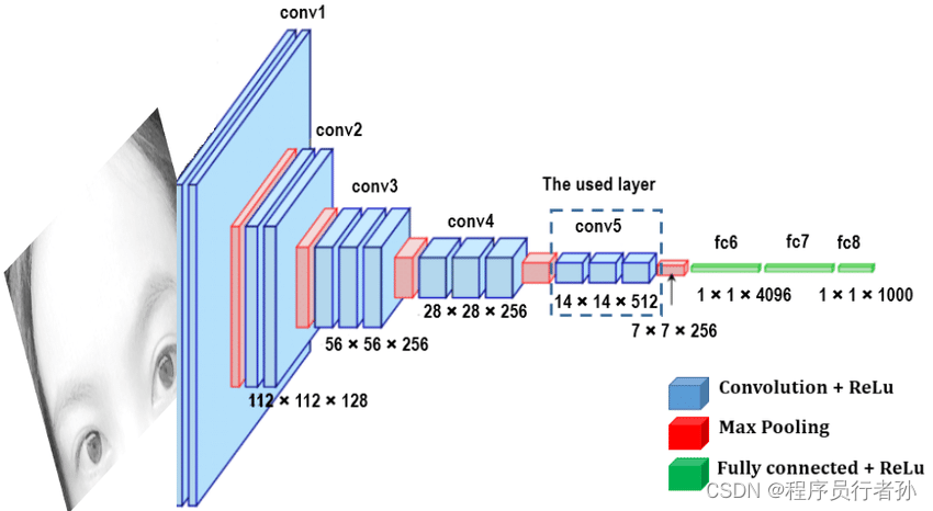
2. MobileNet v1网络结构
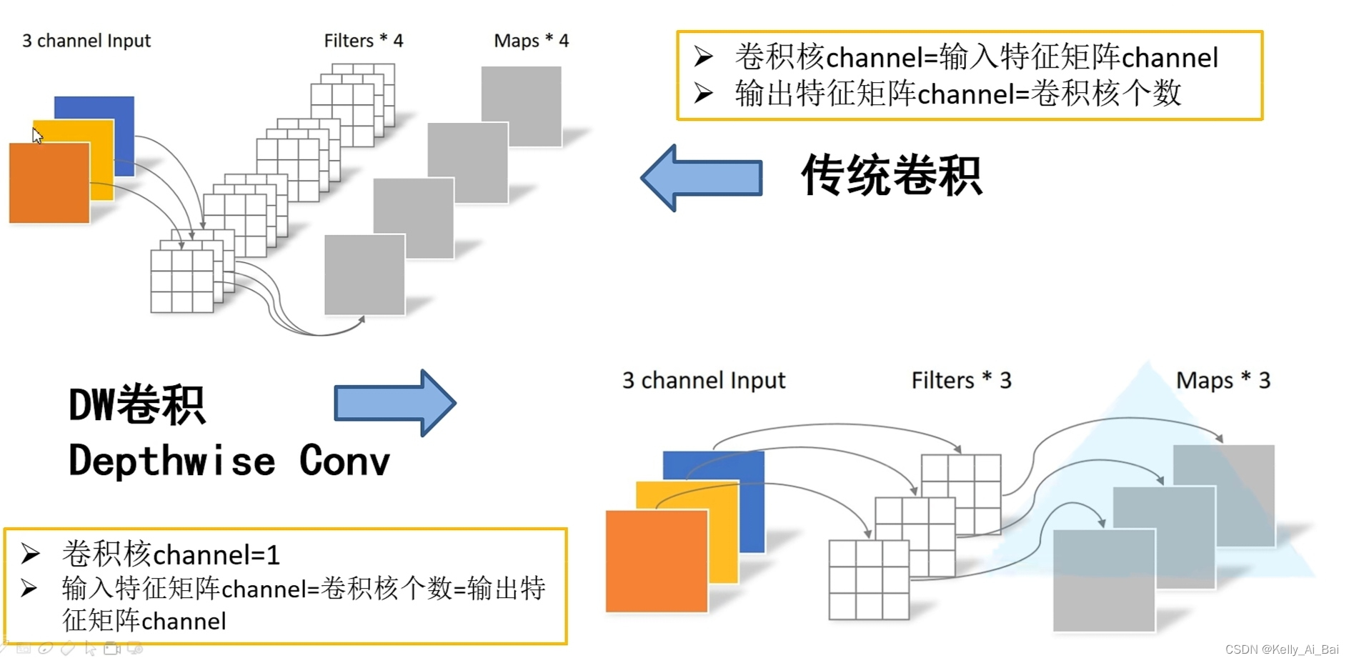
关于深度可分离卷积的详细介绍,可参考另一篇博客:深入浅出理解深度可分离卷积(Depthwise Separable Convolution)

3. (PyTorch)代码实现
3.1 搭建MobileNet v1网络模型
import torch.nn as nn


# MobileNet v1
class MobileNetV1(nn.Module):
    def __init__(self,num_classes=1000):
        super(MobileNetV1, self).__init__()

        # 第一层的卷积,channel->32,size减半
        def conv_bn(in_channel, out_channel, stride):
            return nn.Sequential(
                nn.Conv2d(in_channel, out_channel, 3, stride, 1, bias=False),
                nn.BatchNorm2d(out_channel),
                nn.ReLU(inplace=True)
            )

        # 深度可分离卷积=depthwise卷积 + pointwise卷积
        def conv_dw(in_channel, out_channel, stride):
            return nn.Sequential(
                # depthwise 卷积,channel不变,stride = 2的时候,size减半
                nn.Conv2d(in_channel, in_channel, 3, stride, padding=1, groups=in_channel, bias=False),
                nn.BatchNorm2d(in_channel),
                nn.ReLU(inplace=True),

                # pointwise卷积(1*1卷积) same卷积, 只改变channel
                nn.Conv2d(in_channel, out_channel, 1, 1, padding=0, bias=False),
                nn.BatchNorm2d(out_channel),
                nn.ReLU(inplace=True),
            )

        self.model = nn.Sequential(
            conv_bn(3, 32, 2),          # conv/s2           out=224*224*32
            conv_dw(32, 64, 1),         # conv dw +1*1      out=112*112*64
            conv_dw(64, 128, 2),        # conv dw +1*1      out=56*56*128
            conv_dw(128, 128, 1),       # conv dw +1*1      out=56*56*128
            conv_dw(128, 256, 2),       # conv dw +1*1      out=28*28*256
            conv_dw(256, 256, 1),       # conv dw +1*1      out=28*28*256
            conv_dw(256, 512, 2),       # conv dw +1*1      out=14*14*512
            conv_dw(512, 512, 1),       # 5个 conv dw +1*1 ----> size不变,channel不变,out=14*14*512
            conv_dw(512, 512, 1),
            conv_dw(512, 512, 1),
            conv_dw(512, 512, 1),
            conv_dw(512, 512, 1),
            conv_dw(512, 1024, 2),      # conv dw +1*1      out=7*7*1024
            conv_dw(1024, 1024, 1),     # conv dw +1*1      out=7*7*1024
            nn.AvgPool2d(7),            # avg pool          out=1*1*1024
        )
        self.fc = nn.Linear(1024, num_classes)      # fc

    def forward(self, x):
        x = self.model(x)
        x = x.view(-1, 1024)
        x = self.fc(x)
        return x
3.2 torchsummary查看网络结构
# 安装torchsummary
pip install torchsummary
使用 torchsummary 查看网络结构:
from torchsummary import summary
import torch


DEVICE = 'cuda' if torch.cuda.is_available() else 'cpu'
net = MobileNetV1()
net.to(DEVICE)
print(summary(net, input_size=(3, 224, 224),device=DEVICE))
输出结果
----------------------------------------------------------------
        Layer (type)               Output Shape         Param #
================================================================
            Conv2d-1         [-1, 32, 112, 112]             864
       BatchNorm2d-2         [-1, 32, 112, 112]              64
              ReLU-3         [-1, 32, 112, 112]               0
            Conv2d-4         [-1, 32, 112, 112]             288
       BatchNorm2d-5         [-1, 32, 112, 112]              64
              ReLU-6         [-1, 32, 112, 112]               0
            Conv2d-7         [-1, 64, 112, 112]           2,048
       BatchNorm2d-8         [-1, 64, 112, 112]             128
              ReLU-9         [-1, 64, 112, 112]               0
           Conv2d-10           [-1, 64, 56, 56]             576
      BatchNorm2d-11           [-1, 64, 56, 56]             128
             ReLU-12           [-1, 64, 56, 56]               0
           Conv2d-13          [-1, 128, 56, 56]           8,192
      BatchNorm2d-14          [-1, 128, 56, 56]             256
             ReLU-15          [-1, 128, 56, 56]               0
           Conv2d-16          [-1, 128, 56, 56]           1,152
      BatchNorm2d-17          [-1, 128, 56, 56]             256
             ReLU-18          [-1, 128, 56, 56]               0
           Conv2d-19          [-1, 128, 56, 56]          16,384
      BatchNorm2d-20          [-1, 128, 56, 56]             256
             ReLU-21          [-1, 128, 56, 56]               0
           Conv2d-22          [-1, 128, 28, 28]           1,152
      BatchNorm2d-23          [-1, 128, 28, 28]             256
             ReLU-24          [-1, 128, 28, 28]               0
           Conv2d-25          [-1, 256, 28, 28]          32,768
      BatchNorm2d-26          [-1, 256, 28, 28]             512
             ReLU-27          [-1, 256, 28, 28]               0
           Conv2d-28          [-1, 256, 28, 28]           2,304
      BatchNorm2d-29          [-1, 256, 28, 28]             512
             ReLU-30          [-1, 256, 28, 28]               0
           Conv2d-31          [-1, 256, 28, 28]          65,536
      BatchNorm2d-32          [-1, 256, 28, 28]             512
             ReLU-33          [-1, 256, 28, 28]               0
           Conv2d-34          [-1, 256, 14, 14]           2,304
      BatchNorm2d-35          [-1, 256, 14, 14]             512
             ReLU-36          [-1, 256, 14, 14]               0
           Conv2d-37          [-1, 512, 14, 14]         131,072
      BatchNorm2d-38          [-1, 512, 14, 14]           1,024
             ReLU-39          [-1, 512, 14, 14]               0
           Conv2d-40          [-1, 512, 14, 14]           4,608
      BatchNorm2d-41          [-1, 512, 14, 14]           1,024
             ReLU-42          [-1, 512, 14, 14]               0
           Conv2d-43          [-1, 512, 14, 14]         262,144
      BatchNorm2d-44          [-1, 512, 14, 14]           1,024
             ReLU-45          [-1, 512, 14, 14]               0
           Conv2d-46          [-1, 512, 14, 14]           4,608
      BatchNorm2d-47          [-1, 512, 14, 14]           1,024
             ReLU-48          [-1, 512, 14, 14]               0
           Conv2d-49          [-1, 512, 14, 14]         262,144
      BatchNorm2d-50          [-1, 512, 14, 14]           1,024
             ReLU-51          [-1, 512, 14, 14]               0
           Conv2d-52          [-1, 512, 14, 14]           4,608
      BatchNorm2d-53          [-1, 512, 14, 14]           1,024
             ReLU-54          [-1, 512, 14, 14]               0
           Conv2d-55          [-1, 512, 14, 14]         262,144
      BatchNorm2d-56          [-1, 512, 14, 14]           1,024
             ReLU-57          [-1, 512, 14, 14]               0
           Conv2d-58          [-1, 512, 14, 14]           4,608
      BatchNorm2d-59          [-1, 512, 14, 14]           1,024
             ReLU-60          [-1, 512, 14, 14]               0
           Conv2d-61          [-1, 512, 14, 14]         262,144
      BatchNorm2d-62          [-1, 512, 14, 14]           1,024
             ReLU-63          [-1, 512, 14, 14]               0
           Conv2d-64          [-1, 512, 14, 14]           4,608
      BatchNorm2d-65          [-1, 512, 14, 14]           1,024
             ReLU-66          [-1, 512, 14, 14]               0
           Conv2d-67          [-1, 512, 14, 14]         262,144
      BatchNorm2d-68          [-1, 512, 14, 14]           1,024
             ReLU-69          [-1, 512, 14, 14]               0
           Conv2d-70            [-1, 512, 7, 7]           4,608
      BatchNorm2d-71            [-1, 512, 7, 7]           1,024
             ReLU-72            [-1, 512, 7, 7]               0
           Conv2d-73           [-1, 1024, 7, 7]         524,288
      BatchNorm2d-74           [-1, 1024, 7, 7]           2,048
             ReLU-75           [-1, 1024, 7, 7]               0
           Conv2d-76           [-1, 1024, 7, 7]           9,216
      BatchNorm2d-77           [-1, 1024, 7, 7]           2,048
             ReLU-78           [-1, 1024, 7, 7]               0
           Conv2d-79           [-1, 1024, 7, 7]       1,048,576
      BatchNorm2d-80           [-1, 1024, 7, 7]           2,048
             ReLU-81           [-1, 1024, 7, 7]               0
        AvgPool2d-82           [-1, 1024, 1, 1]               0
           Linear-83                 [-1, 1000]       1,025,000
================================================================
Total params: 4,231,976
Trainable params: 4,231,976
Non-trainable params: 0
----------------------------------------------------------------
Input size (MB): 0.57
Forward/backward pass size (MB): 115.43
Params size (MB): 16.14
Estimated Total Size (MB): 132.15
----------------------------------------------------------------
None
3.3 train训练模型
import torch
import torch.nn as nn
from torchvision import transforms, datasets
import torch.optim as optim
from model import MobileNetV1
from torch.utils.data import DataLoader
from tqdm import tqdm

DEVICE = 'cuda' if torch.cuda.is_available() else 'cpu'
data_transform = {

    "train": transforms.Compose([transforms.Resize((224, 224)),
                                 transforms.ToTensor(),
                                 transforms.Normalize([0.485, 0.456, 0.406], [0.229, 0.224, 0.255])]),
    "test": transforms.Compose([transforms.Resize((224, 224)),
                                transforms.ToTensor(),
                                transforms.Normalize([0.485, 0.456, 0.406], [0.229, 0.224, 0.255])])}

# 训练集
trainset = datasets.CIFAR10(root='./data', train=True, download=True, transform=data_transform['train'])
trainloader = DataLoader(trainset, batch_size=16, shuffle=True)

# 测试集
testset = datasets.CIFAR10(root='./data', train=False, download=True, transform=data_transform['test'])
testloader = DataLoader(testset, batch_size=16, shuffle=False)

# 样本的个数
num_trainset = len(trainset)  # 50000
num_testset = len(testset)  # 10000

# 构建网络
net = MobileNetV1(num_classes=10)
net.to(DEVICE)

# 加载损失和优化器
loss_function = nn.CrossEntropyLoss()
loss_fun = loss_function.to(DEVICE)

learning_rate = 0.0001
optimizer = optim.Adam(net.parameters(), lr=learning_rate)

best_acc = 0.0
save_path = './MobileNetV1.pth'

for epoch in range(10):
    net.train()  # 训练模式
    running_loss = 0.0
    for data in tqdm(trainloader):
        images, labels = data
        images, labels = images.to(DEVICE), labels.to(DEVICE)

        optimizer.zero_grad()
        out = net(images)  # 总共有三个输出
        loss = loss_function(out, labels)
        loss.backward()  # 反向传播
        optimizer.step()

        running_loss += loss.item()

    # test
    # 测试过程不需要通过反向传播来更新参数。
    net.eval()  # 测试模式
    acc = 0.0
    with torch.no_grad():  # 测试不需要进行反向传播,即不需要梯度变化
        for test_data in tqdm(testloader):
            test_images, test_labels = test_data
            test_images, test_labels = test_images.to(DEVICE), test_labels.to(DEVICE)

            outputs = net(test_images)
            predict_y = torch.max(outputs, dim=1)[1]
            acc += (predict_y == test_labels).sum().item()

    accurate = acc / num_testset
    train_loss = running_loss / num_trainset

    print('[epoch %d] train_loss: %.3f  test_accuracy: %.3f' %
          (epoch + 1, train_loss, accurate))

    if accurate > best_acc:
        best_acc = accurate
        torch.save(net.state_dict(), save_path)

print('Finished Training')
输出结果
Downloading https://www.cs.toronto.edu/~kriz/cifar-10-python.tar.gz to ./data/cifar-10-python.tar.gz
170499072it [00:30, 5634555.25it/s]
Extracting ./data/cifar-10-python.tar.gz to ./data
Files already downloaded and verified
100%|██████████| 3125/3125 [02:18<00:00, 22.55it/s]
100%|██████████| 625/625 [00:12<00:00, 51.10it/s]
[epoch 1] train_loss: 0.101  test_accuracy: 0.516
100%|██████████| 3125/3125 [02:23<00:00, 21.78it/s]
100%|██████████| 625/625 [00:11<00:00, 54.31it/s]
[epoch 2] train_loss: 0.079  test_accuracy: 0.612
100%|██████████| 3125/3125 [02:20<00:00, 22.17it/s]
100%|██████████| 625/625 [00:11<00:00, 54.28it/s]
[epoch 3] train_loss: 0.066  test_accuracy: 0.672
100%|██████████| 3125/3125 [02:21<00:00, 22.09it/s]
100%|██████████| 625/625 [00:11<00:00, 55.52it/s]
[epoch 4] train_loss: 0.056  test_accuracy: 0.722
100%|██████████| 3125/3125 [02:13<00:00, 23.34it/s]
100%|██████████| 625/625 [00:11<00:00, 55.56it/s]
[epoch 5] train_loss: 0.048  test_accuracy: 0.748
100%|██████████| 3125/3125 [02:14<00:00, 23.31it/s]
100%|██████████| 625/625 [00:11<00:00, 52.19it/s]
[epoch 6] train_loss: 0.042  test_accuracy: 0.763
100%|██████████| 3125/3125 [02:14<00:00, 23.18it/s]
100%|██████████| 625/625 [00:11<00:00, 56.05it/s]
[epoch 7] train_loss: 0.035  test_accuracy: 0.781
100%|██████████| 3125/3125 [02:14<00:00, 23.27it/s]
100%|██████████| 625/625 [00:11<00:00, 55.88it/s]
[epoch 8] train_loss: 0.031  test_accuracy: 0.790
100%|██████████| 3125/3125 [02:13<00:00, 23.32it/s]
100%|██████████| 625/625 [00:11<00:00, 55.89it/s]
[epoch 9] train_loss: 0.026  test_accuracy: 0.801
100%|██████████| 3125/3125 [02:15<00:00, 22.99it/s]
100%|██████████| 625/625 [00:11<00:00, 55.95it/s]
[epoch 10] train_loss: 0.022  test_accuracy: 0.803
Finished Training

Process finished with exit code 0
显卡资源占用情况

3.4 查看模型权重参数
from model import MobileNetV1
import torch


DEVICE = 'cuda' if torch.cuda.is_available() else 'cpu'

net = MobileNetV1(num_classes=10)
net.load_state_dict(torch.load('./MobileNetV1.pth'))
net.to(DEVICE)


with torch.no_grad():
    for i in range(0,14):       # 查看 depthwise 的权值
        print(net.model[i][0].weight)
3.5 在CIFAR10数据集上测试效果
import os
os.environ['KMP_DUPLICATE_LIB_OK'] = 'True'

import torch
import numpy as np
import matplotlib.pyplot as plt
from model import MobileNetV1
from torchvision.transforms import transforms
from torch.utils.data import DataLoader
import torchvision

classes = ('plane', 'car', 'bird', 'cat', 'deer', 'dog', 'frog', 'horse', 'ship', 'truck')

# 预处理
transformer = transforms.Compose([transforms.Resize((224,224)),
                                  transforms.ToTensor(),
                                  transforms.Normalize([0.485, 0.456, 0.406], [0.229, 0.224, 0.255])])

# 加载模型
DEVICE = 'cuda' if torch.cuda.is_available() else 'cpu'
model = MobileNetV1(num_classes=10)
model.load_state_dict(torch.load('./MobileNetV1.pth'))
model.to(DEVICE)

# 加载数据
testSet = torchvision.datasets.CIFAR10(root='./data', train=False, download=False, transform=transformer)
testLoader = DataLoader(testSet, batch_size=12, shuffle=True)

# 获取一批数据
imgs, labels = next(iter(testLoader))
imgs = imgs.to(DEVICE)

# show
with torch.no_grad():
    model.eval()
    prediction = model(imgs)  # 预测
    prediction = torch.max(prediction, dim=1)[1]
    prediction = prediction.data.cpu().numpy()

    plt.figure(figsize=(12, 8))
    for i, (img, label) in enumerate(zip(imgs, labels)):
        x = np.transpose(img.data.cpu().numpy(), (1, 2, 0))  # 图像
        x[:, :, 0] = x[:, :, 0] * 0.229 + 0.485  # 去 normalization
        x[:, :, 1] = x[:, :, 1] * 0.224 + 0.456  # 去 normalization
        x[:, :, 2] = x[:, :, 2] * 0.255 + 0.406  # 去 normalization
        y = label.numpy().item()  # label
        plt.subplot(3, 4, i + 1)
        plt.axis(False)
        plt.imshow(x)
        plt.title('R:{},P:{}'.format(classes[y], classes[prediction[i]]))
    plt.show()
结果展示

三、MobileNet v2
原始论文:[2]
1. 引言
特征图的每个通道的像素值所代表的特征可以映射到一个低维子空间的流形区域上。通常,在进行卷积操作之后往往会接一层激活层,以此增加特征的非线性,一个常见的激活函数就是 ReLU。激活过程会带来信息损耗,而且这种损耗是无法恢复的,当通道数非常少时,ReLU 的信息损耗更为明显。
如下图所示,其输入是一个表示流形数据的矩阵,和卷积操作类似,经过 n 个ReLU的操作得到 n 个通道的Feature Map,然后通过 n 个Feature Map还原输入数据,还原的越像说明信息损耗的越少。

从上图可以看出,在输入维度是2,3时,输出和输入相比丢失了较多信息;但是在输入维度是15到30时,输出则保留了输入的较多信息。总得来说,当n值较小时,ReLU的信息损耗非常严重,当n值较大时,输入流形能较好还原。
根据对上面提到的信息损耗问题分析,我们可以有两种解决方案:
- 替换ReLU:既然是
ReLU导致的信息损耗,那么可以将ReLU替换成线性激活函数; - 提高维度:如果比较多的通道数能减少信息损耗,那么可以通过升维将输入的维度变高。
MobileNet v2的题目为 MobileNetV2: Inverted Residuals and Linear Bottlenecks , Linear Bottlenecks 和 Inverted Residuals 就是MobileNet v2的核心,分别对应上述两种思路。
2. MobileNet v2创新点
MobileNet v2主要是将残差网络和深度可分离卷积(Depthwise Separable Convolution)进行结合,通过分析单通道的流形特征对残差块进行改进,包括对中间层的扩展(d)以及 bottleneck layers 的线性激活©。

2.1 Linear Bottlenecks
将 Relu 激活函数替换为线性激活函数,文章中将变换后的块称为 Linear Bottlenecks,结构如下图所示:

当然不能把 ReLU 全部替换为线性激活函数,不然网络将会退化为单层神经网络,一个折中方案是在输出 feature map 的通道数较少的时候,也就是 bottleneck 部分使用线性激活函数,其它时候使用 ReLU。Linear Bottlenecks 块的代码实现如下:
def _bottleneck(inputs, nb_filters, t):
    x = Conv2D(filters=nb_filters * t, kernel_size=(1,1), padding='same')(inputs)
    x = Activation(relu6)(x)
    x = DepthwiseConv2D(kernel_size=(3,3), padding='same')(x)
    x = Activation(relu6)(x)
    x = Conv2D(filters=nb_filters, kernel_size=(1,1), padding='same')(x)
    # do not use activation function
    if not K.get_variable_shape(inputs)[3] == nb_filters:
        inputs = Conv2D(filters=nb_filters, kernel_size=(1,1), padding='same')(inputs)
    outputs = add([x, inputs])
    return outputs
2. 3Inverted Residual
Inverted Residuals直译为倒残差结构,我们来看看其与正常的残差结构有什么区别和联系:通过下图可以看出,左侧为ResNet中的残差结构,其结构为:1x1卷积降维->3x3卷积->1x1卷积升维;右侧为MobileNet v2中的倒残差结构,其结构为:1x1卷积升维->3x3DW卷积->1x1卷积降维。MobileNet v2先使用 1x1 的卷积进行升维的原因是:高维信息通过ReLU激活函数后丢失的信息更少,因此先进行升维操作。

这部分需要注意的是只有当步长s=1时,才有shortcut连接,步长为2是没有的,如下图所示。

3. MobileNet v2网络结构

MobileNet v2所用的参数更少,但mAP值和其它的差不多,甚至超过了Yolov2,其效果如下图所示:

4. 代码实现
MobileNet v2的实现可以通过堆叠 bottleneck 的形式实现,如下面代码片段:
def MobileNetV2_relu(input_shape, k):
    inputs = Input(shape = input_shape)
    x = Conv2D(filters=32, kernel_size=(3,3), padding='same')(inputs)
    x = _bottleneck_relu(x, 8, 6)
    x = MaxPooling2D((2,2))(x)
    x = _bottleneck_relu(x, 16, 6)
    x = _bottleneck_relu(x, 16, 6)
    x = MaxPooling2D((2,2))(x)
    x = _bottleneck_relu(x, 32, 6)
    x = GlobalAveragePooling2D()(x)
    x = Dense(128, activation='relu')(x)
    outputs = Dense(k, activation='softmax')(x)
    model = Model(inputs, outputs)
    return model


![[Python图像处理] 使用OpenCV创建深度图](https://img-blog.csdnimg.cn/9760aa8ef2ca480b8a169f897a1e3f4e.png)