0 前言
无人驾驶技术是机器学习为主的一门前沿领域,在无人驾驶领域中机器学习的各种算法随处可见,今天学长给大家介绍无人驾驶技术中的车道线检测。
1 车道线检测
在无人驾驶领域每一个任务都是相当复杂,看上去无从下手。那么面对这样极其复杂问题,我们解决问题方式从先尝试简化问题,然后由简入难一步一步尝试来一个一个地解决问题。车道线检测在无人驾驶中应该算是比较简单的任务,依赖计算机视觉一些相关技术,通过读取
camera 传入的图像数据进行分析,识别出车道线位置,我想这个对于 lidar
可能是无能为力。所以今天我们就从最简单任务说起,看看有哪些技术可以帮助我们检出车道线。
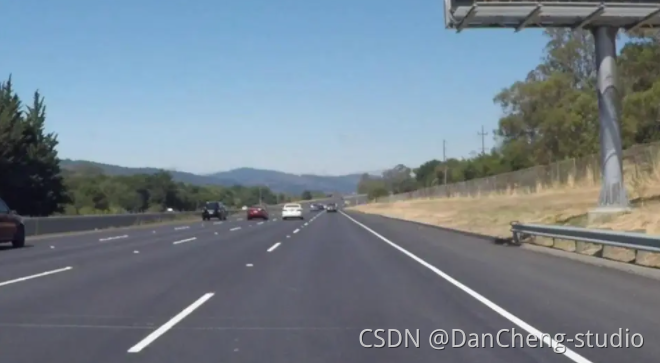
我们先把问题简化,所谓简化问题就是用一些条件限制来缩小车道线检测的问题。我们先看数据,也就是输入算法是车辆行驶的图像,输出车道线位置。
更多时候我们如何处理一件比较困难任务,可能有时候我们拿到任务时还没有任何思路,不要着急也不用想太多,我们先开始一步一步地做,从最简单的开始做起,随着做就会有思路,同样一些问题也会暴露出来。我们先找一段视频,这段视频是我从网上一个关于车道线检测项目中拿到的,也参考他的思路来做这件事。好现在就开始做这件事,那么最简单的事就是先读取视频,然后将其显示在屏幕以便于调试。
2 目标
检测图像中车道线位置,将车道线信息提供路径规划。
3 检测思路
- 图像灰度处理
- 图像高斯平滑处理
- canny 边缘检测
- 区域 Mask
- 霍夫变换
- 绘制车道线
4 代码实现
4.1 视频图像加载
import cv2
import numpy as np
import sys
import pygame
from pygame.locals import *
class Display(object):
def __init__(self,Width,Height):
pygame.init()
pygame.display.set_caption('Drive Video')
self.screen = pygame.display.set_mode((Width,Height),0,32)
def paint(self,draw):
self.screen.fill([0,0,0])
draw = cv2.transpose(draw)
draw = pygame.surfarray.make_surface(draw)
self.screen.blit(draw,(0,0))
pygame.display.update()
if __name__ == "__main__":
solid_white_right_video_path = "test_videos/丹成学长车道线检测.mp4"
cap = cv2.VideoCapture(solid_white_right_video_path)
Width = int(cap.get(cv2.CAP_PROP_FRAME_WIDTH))
Height = int(cap.get(cv2.CAP_PROP_FRAME_HEIGHT))
display = Display(Width,Height)
while True:
ret, draw = cap.read()
draw = cv2.cvtColor(draw,cv2.COLOR_BGR2RGB)
if ret == False:
break
display.paint(draw)
for event in pygame.event.get():
if event.type == QUIT:
sys.exit()
上面代码学长就不多说了,默认大家对 python 是有所了解,关于如何使用 opencv 读取图片网上代码示例也很多,大家一看就懂。这里因为我用的是 mac
有时候显示视频图像可能会有些问题,所以我们用 pygame 来显示 opencv 读取图像。这个大家根据自己实际情况而定吧。值得说一句的是 opencv
读取图像是 BGR 格式,要想在 pygame 中正确显示图像就需要将 BGR 转换为 RGB 格式。
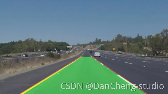
4.2 车道线区域
现在这个区域是我们根据观测图像绘制出来,
 def color_select(img,red_threshold=200,green_threshold=200,blue_threshold=200):
        ysize,xsize = img.shape[:2]


        color_select = np.copy(img)

        rgb_threshold = [red_threshold, green_threshold, blue_threshold]

        thresholds = (img[:,:,0] < rgb_threshold[0]) \
                | (img[:,:,1] < rgb_threshold[1]) \
                | (img[:,:,2] < rgb_threshold[2])
        color_select[thresholds] = [0,0,0]

        return color_select
效果如下:
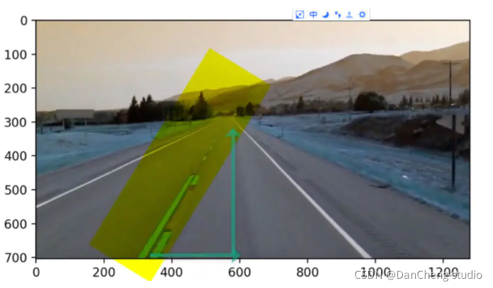
4.3 区域
我们要检测车道线位置相对比较固定,通常出现车的前方,所以我们通过绘制,也就是仅检测我们关心区域。通过创建 mask 来过滤掉那些不关心的区域保留关心区域。
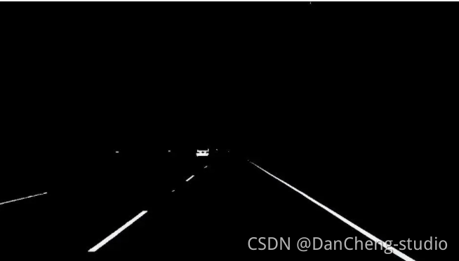
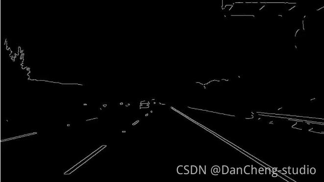
4.4 canny 边缘检测
有关边缘检测也是计算机视觉。首先利用梯度变化来检测图像中的边,如何识别图像的梯度变化呢,答案是卷积核。卷积核是就是不连续的像素上找到梯度变化较大位置。我们知道
sobal 核可以很好检测边缘,那么 canny 就是 sobal 核检测上进行优化。
# 示例代码,作者丹成学长:Q746876041
def canny_edge_detect(img):
gray = cv2.cvtColor(img,cv2.COLOR_RGB2GRAY)
kernel_size = 5
blur_gray = cv2.GaussianBlur(gray,(kernel_size, kernel_size),0)
low_threshold = 180
high_threshold = 240
edges = cv2.Canny(blur_gray, low_threshold, high_threshold)
return edges
4.5 霍夫变换(Hough transform)
霍夫变换是将 x 和 y 坐标系中的线映射表示在霍夫空间的点(m,b)。所以霍夫变换实际上一种由繁到简(类似降维)的操作。当使用 canny
进行边缘检测后图像可以交给霍夫变换进行简单图形(线、圆)等的识别。这里用霍夫变换在 canny 边缘检测结果中寻找直线。
ignore_mask_color = 255
# 获取图片尺寸
imshape = img.shape
# 定义 mask 顶点
vertices = np.array([[(0,imshape[0]),(450, 290), (490, 290), (imshape[1],imshape[0])]], dtype=np.int32)
# 使用 fillpoly 来绘制 mask
cv2.fillPoly(mask, vertices, ignore_mask_color)
masked_edges = cv2.bitwise_and(edges, mask)
# 定义Hough 变换的参数
rho = 1
theta = np.pi/180
threshold = 2
min_line_length = 4 # 组成一条线的最小像素数
max_line_gap = 5 # 可连接线段之间的最大像素间距
# 创建一个用于绘制车道线的图片
line_image = np.copy(img)*0
# 对于 canny 边缘检测结果应用 Hough 变换
# 输出“线”是一个数组,其中包含检测到的线段的端点
lines = cv2.HoughLinesP(masked_edges, rho, theta, threshold, np.array([]),
min_line_length, max_line_gap)
# 遍历“线”的数组来在 line_image 上绘制
for line in lines:
for x1,y1,x2,y2 in line:
cv2.line(line_image,(x1,y1),(x2,y2),(255,0,0),10)
color_edges = np.dstack((edges, edges, edges))
import math
import cv2
import numpy as np
"""
Gray Scale
Gaussian Smoothing
Canny Edge Detection
Region Masking
Hough Transform
Draw Lines [Mark Lane Lines with different Color]
"""
class SimpleLaneLineDetector(object):
def __init__(self):
pass
def detect(self,img):
# 图像灰度处理
gray_img = self.grayscale(img)
print(gray_img)
#图像高斯平滑处理
smoothed_img = self.gaussian_blur(img = gray_img, kernel_size = 5)
#canny 边缘检测
canny_img = self.canny(img = smoothed_img, low_threshold = 180, high_threshold = 240)
#区域 Mask
masked_img = self.region_of_interest(img = canny_img, vertices = self.get_vertices(img))
#霍夫变换
houghed_lines = self.hough_lines(img = masked_img, rho = 1, theta = np.pi/180, threshold = 20, min_line_len = 20, max_line_gap = 180)
# 绘制车道线
output = self.weighted_img(img = houghed_lines, initial_img = img, alpha=0.8, beta=1., gamma=0.)
return output
def grayscale(self,img):
return cv2.cvtColor(img, cv2.COLOR_RGB2GRAY)
def canny(self,img, low_threshold, high_threshold):
return cv2.Canny(img, low_threshold, high_threshold)
def gaussian_blur(self,img, kernel_size):
return cv2.GaussianBlur(img, (kernel_size, kernel_size), 0)
def region_of_interest(self,img, vertices):
mask = np.zeros_like(img)
if len(img.shape) > 2:
channel_count = img.shape[2]
ignore_mask_color = (255,) * channel_count
else:
ignore_mask_color = 255
cv2.fillPoly(mask, vertices, ignore_mask_color)
masked_image = cv2.bitwise_and(img, mask)
return masked_image
def draw_lines(self,img, lines, color=[255, 0, 0], thickness=10):
for line in lines:
for x1,y1,x2,y2 in line:
cv2.line(img, (x1, y1), (x2, y2), color, thickness)
def slope_lines(self,image,lines):
img = image.copy()
poly_vertices = []
order = [0,1,3,2]
left_lines = []
right_lines = []
for line in lines:
for x1,y1,x2,y2 in line:
if x1 == x2:
pass
else:
m = (y2 - y1) / (x2 - x1)
c = y1 - m * x1
if m < 0:
left_lines.append((m,c))
elif m >= 0:
right_lines.append((m,c))
left_line = np.mean(left_lines, axis=0)
right_line = np.mean(right_lines, axis=0)
for slope, intercept in [left_line, right_line]:
rows, cols = image.shape[:2]
y1= int(rows)
y2= int(rows*0.6)
x1=int((y1-intercept)/slope)
x2=int((y2-intercept)/slope)
poly_vertices.append((x1, y1))
poly_vertices.append((x2, y2))
self.draw_lines(img, np.array([[[x1,y1,x2,y2]]]))
poly_vertices = [poly_vertices[i] for i in order]
cv2.fillPoly(img, pts = np.array([poly_vertices],'int32'), color = (0,255,0))
return cv2.addWeighted(image,0.7,img,0.4,0.)
def hough_lines(self,img, rho, theta, threshold, min_line_len, max_line_gap):
lines = cv2.HoughLinesP(img, rho, theta, threshold, np.array([]), minLineLength=min_line_len, maxLineGap=max_line_gap)
line_img = np.zeros((img.shape[0], img.shape[1], 3), dtype=np.uint8)
line_img = self.slope_lines(line_img,lines)
return line_img
def weighted_img(self,img, initial_img, alpha=0.1, beta=1., gamma=0.):
lines_edges = cv2.addWeighted(initial_img, alpha, img, beta, gamma)
return lines_edges
def get_vertices(self,image):
rows, cols = image.shape[:2]
bottom_left = [cols*0.15, rows]
top_left = [cols*0.45, rows*0.6]
bottom_right = [cols*0.95, rows]
top_right = [cols*0.55, rows*0.6]
ver = np.array([[bottom_left, top_left, top_right, bottom_right]], dtype=np.int32)
return ver
4.6 HoughLinesP 检测原理
接下来进入代码环节,学长详细给大家解释一下 HoughLinesP 参数的含义以及如何使用。
lines = cv2.HoughLinesP(cropped_image,2,np.pi/180,100,np.array([]),minLineLength=40,maxLineGap=5)
- 第一参数是我们要检查的图片 Hough accumulator 数组
- 第二个和第三个参数用于定义我们 Hough 坐标如何划分 bin,也就是小格的精度。我们通过曲线穿过 bin 格子来进行投票,我们根据投票数量来决定 p 和 theta 的值。2 表示我们小格宽度以像素为单位 。
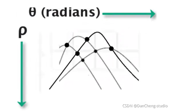
我们可以通过下图划分小格,只要曲线穿过就会对小格进行投票,我们记录投票数量,记录最多的作为参数
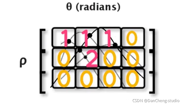
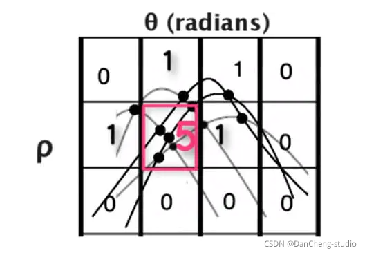
- 如果定义尺寸过大也就失去精度,如果定义格子尺寸过小虽然精度上来了,这样也会打来增长计算时间。
- 接下来参数 100 表示我们投票为 100 以上的线才是符合要求是我们要找的线。也就是在 bin 小格子需要有 100 以上线相交于此才是我们要找的参数。
- minLineLength 给 40 表示我们检查线长度不能小于 40 pixel
- maxLineGap=5 作为线间断不能大于 5 pixel
4.6.1 定义显示车道线方法
def disply_lines(image,lines):
pass
通过定义函数将找到的车道线显示出来。
line_image = disply_lines(lane_image,lines)
4.6.2 查看探测车道线数据结构
def disply_lines(image,lines):
line_image = np.zeros_like(image)
if lines is not None:
for line in lines:
print(line)
先定义一个尺寸大小和原图一样的矩阵用于绘制查找到车道线,我们先判断一下是否已经找到车道线,lines 返回值应该不为 None
是一个矩阵,我们可以简单地打印一下看一下效果
[[704 418 927 641]]
[[704 426 791 516]]
[[320 703 445 494]]
[[585 301 663 381]]
[[630 341 670 383]]
4.6.3 探测车道线
看数据结构[[x1,y1,x2,y2]] 的二维数组,这就需要我们转换一下为一维数据[x1,y1,x2,y2]
def disply_lines(image,lines):
line_image = np.zeros_like(image)
if liness is not None:
for line in lines:
x1,y1,x2,y2 = line.reshape(4)
cv2.line(line_image,(x1,y1),(x2,y2),(255,0,0),10)
return line_image
line_image = disply_lines(lane_image,lines)
cv2.imshow('result',line_image)
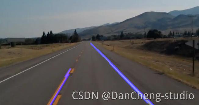
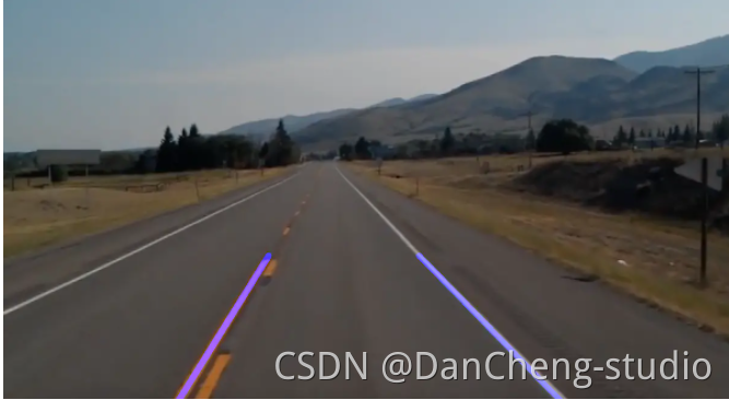
4.6.4 合成
有关合成图片我们是将两张图片通过给一定权重进行叠加合成。

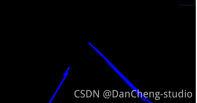
4.6.5 优化
探测到的车道线还是不够平滑,我们需要优化,基本思路就是对这些直线的斜率和截距取平均值然后将所有探测出点绘制到一条直线上。
  def average_slope_intercept(image,lines):
        left_fit = []
        right_fit = []
        for line in lines:
            x1, y1, x2, y2 = line.reshape(4)
            parameters = np.polyfit((x1,x2),(y1,y2),1)
            print(parameters)
这里学长定义两个数组 left_fit 和 right_fit 分别用于存放左右两侧车道线的点,我们打印一下 lines 的斜率和截距,通过 numpy
提供 polyfit 方法输入两个点我们就可以得到通过这些点的直线的斜率和截距。
[ 1. -286.]
[ 1.03448276 -302.27586207]
[ -1.672 1238.04 ]
[ 1.02564103 -299.
[ 1.02564103 -299.
def average_slope_intercept(image,lines):
    left_fit = []
    right_fit = []
    for line in lines:
        x1, y1, x2, y2 = line.reshape(4)
        parameters = np.polyfit((x1,x2),(y1,y2),1)
        # print(parameters)
        slope = parameters[0]
        intercept = parameters[1]
        if slope < 0:
            left_fit.append((slope,intercept))
        else:
            right_fit.append((slope,intercept))
        print(left_fit)
        print(right_fit)
我们输出一下图片大小,我们图片是以其左上角作为原点 0 ,0 来开始计算的,所以我们直线从图片底部 700 多向上绘制我们无需绘制全部可以截距一部分即可。
    def make_coordinates(image, line_parameters):
        slope, intercept = line_parameters
        y1 = image.shape[0]
        y2 = int(y1*(3/5))
        x1 = int((y1 - intercept)/slope)
        x2 = int((y2 - intercept)/slope)
        # print(image.shape)
        return np.array([x1,y1,x2,y2])
所以直线开始和终止我们给定 y1,y2 然后通过方程的斜率和截距根据y 算出 x。
averaged_lines = average_slope_intercept(lane_image,lines);
line_image = disply_lines(lane_image,averaged_lines)
combo_image = cv2.addWeighted(lane_image,0.8, line_image, 1, 1,1)
cv2.imshow('result',combo_image)
5 最后
该项目较为新颖,适合作为竞赛课题方向,学长非常推荐!
🧿 更多资料, 项目分享: