1 作业内容描述
1.1 背景
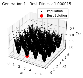
现在有一个函数 3 − s i n 2 ( j x 1 ) − s i n 2 ( j x 2 ) 3-sin^2(jx_1)-sin^2(jx_2) 3−sin2(jx1)−sin2(jx2),有两个变量 x 1 x_1 x1 和 x 2 x_2 x2,它们的定义域为 x 1 , x 2 ∈ [ 0 , 6 ] x_1,x_2\in[0,6] x1,x2∈[0,6],并且 j = 2 j=2 j=2,对于此例,所致对于 j = 2 , 3 , 4 , 5 j=2,3,4,5 j=2,3,4,5分别有 16,36,64,100 个全局最优解。
现在有一个Shubert函数 ∏ i = 1 n ∑ j = 1 5 j cos [ ( j + 1 ) x i + j ] \prod_{i=1}^{n}\sum_{j=1}^{5}j\cos[(j+1)x_i+j] ∏i=1n∑j=15jcos[(j+1)xi+j],其中定义域为 − 10 < x i < 10 -10<x_i<10 −10<xi<10,对于此问题,当n=2时有18个不同的全局最优解
1.2 要求
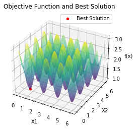
- 求该函数的最小值即 m i n ( 3 − s i n 2 ( j x 1 ) − s i n 2 ( j x 2 ) ) min(3-sin^2(jx_1)-sin^2(jx_2)) min(3−sin2(jx1)−sin2(jx2)),j=2,精确到小数点后6位。
- 求该Shubert函数的最小值即 m i n ( ∏ i = 1 2 ∑ j = 1 5 j cos [ ( j + 1 ) x i + j ] ) min(\prod_{i=1}^{2}\sum_{j=1}^{5}j\cos[(j+1)x_i+j]) min(∏i=12∑j=15jcos[(j+1)xi+j]),精确到小数点后6位
2 作业已完成部分和未完成部分
该作业已经全部完成,没有未完成的部分。
 |
 |
|---|---|
| Colab Notebook | Github Rep |
3. 作业运行结果截图
最后跑出的结果如下:
- 第一个函数的最小值为 1.0000000569262162
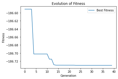
- 第二个函数的最小值为-186.73042323192567
4 核心代码和步骤
4.1 基本的步骤
- 定义目标函数
objective_function:使用了一个二维的目标函数,即 3 − s i n 2 ( j x 1 ) − s i n 2 ( j x 2 ) 3-sin^2(jx_1)-sin^2(jx_2) 3−sin2(jx1)−sin2(jx2)。 - 定义选择函数
crossover:用于交叉操作,通过交叉率(crossover_rate)确定需要进行交
叉的父母对的数量,并在这些父母对中交换某些变量的值。
- 定义变异函数
mutate:用于变异操作,通过变异率(mutation_rate)确定需要进行变异
的父母对的数量,并在这些父母对中随机改变某些变量的值。
- 定义进化算法
evolutionary_algorithm:初始化种群,其中每个个体都是一个二维向量。在
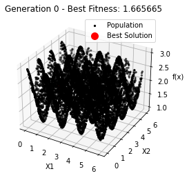
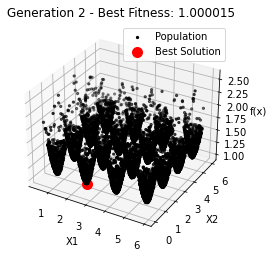
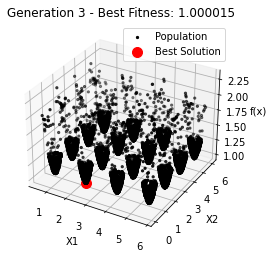
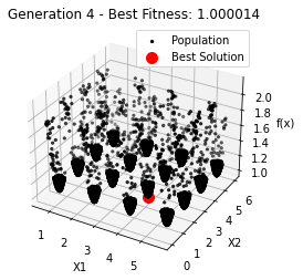
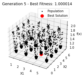
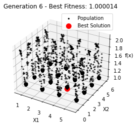
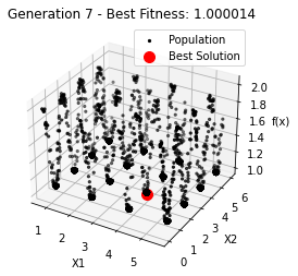
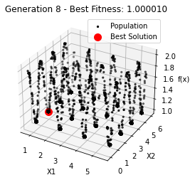
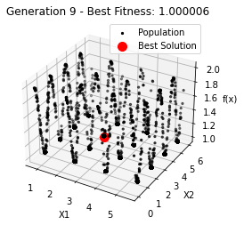
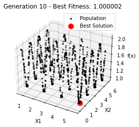
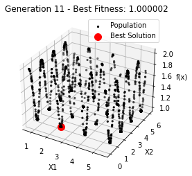
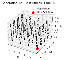
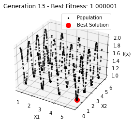
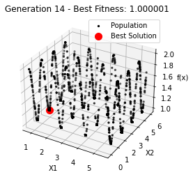
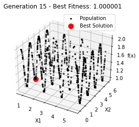
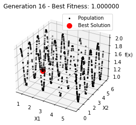
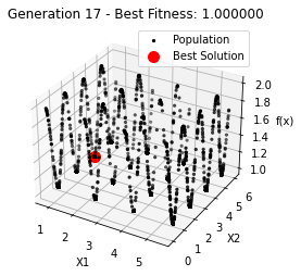
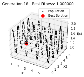
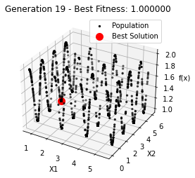
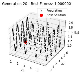
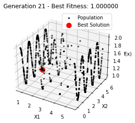
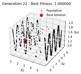
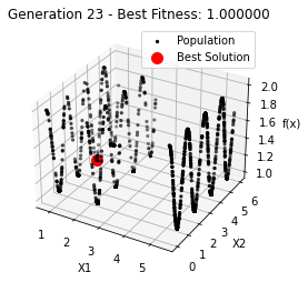
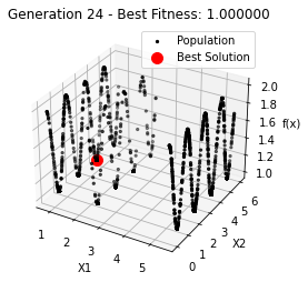
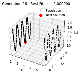
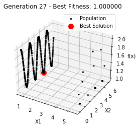
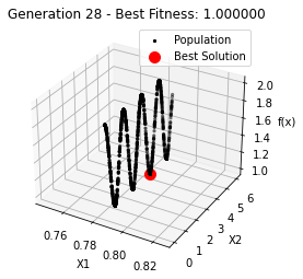
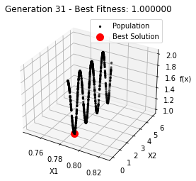
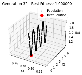
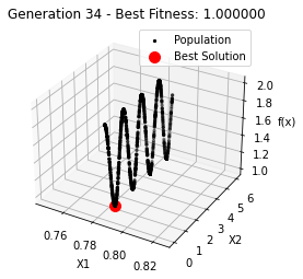
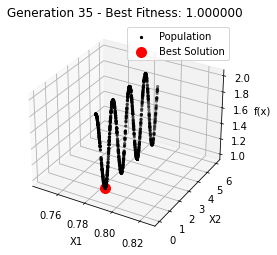
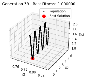
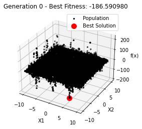
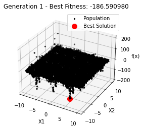
每一代中,计算每个个体的适应度值,绘制三维图表展示种群分布和最佳解。
- 更新全局最佳解。根据适应度值确定复制的数量并形成繁殖池。选择父母、进行交叉和变
异,更新种群。重复上述步骤直到达到指定的迭代次数。
- 设置算法参数:
population_size:种群大小。;num_generations:迭代的次数。;muta
tion_rate:变异率。;crossover_rate:交叉率。
- 运行进化算法
evolutionary_algorithm:调用进化算法函数并获得最终的最佳解、最佳适
应度值和每一代的演化数据。
输出结果:打印最终的最佳解和最佳适应度值。输出每个迭代步骤的最佳适应度值。
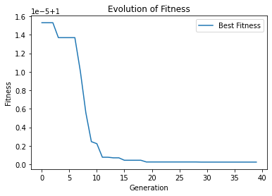
可视化结果:绘制函数曲面和最优解的三维图表。绘制适应度值随迭代次数的变化曲线。
4.2 第一个函数 3 − s i n 2 ( j x 1 ) − s i n 2 ( j x 2 ) 3-sin^2(jx_1)-sin^2(jx_2) 3−sin2(jx1)−sin2(jx2)
import numpy as np
import pandas as pd
import matplotlib.pyplot as plt

# 定义目标函数
def objective_function(x):
    j = 2
    return 3 - np.sin(j * x[0])**2 - np.sin(j * x[1])**2 # 3 - sin(2x1)^2 - sin(2x2)^2

# 定义选择函数
def crossover(parents_1, parents_2, crossover_rate):
    num_parents = len(parents_1) # 父母的数量
    num_crossover = int(crossover_rate * num_parents) # 选择进行交叉的父母对的数量

    # 选择进行交叉的父母对
    crossover_indices = np.random.choice(num_parents, size=num_crossover, replace=False) # 选择进行交叉的父母对的索引

    # 复制父母
    copy_parents_1 = np.copy(parents_1)
    copy_parents_2 = np.copy(parents_2)

    # 进行交叉操作
    for i in crossover_indices:
        parents_1[i][1] = copy_parents_2[i][1] # 交叉变量x2
        parents_2[i][1] = copy_parents_1[i][1] # 交叉变量x2

    return parents_1, parents_2

# 定义变异函数
def mutate(parents_1, parents_2, mutation_rate):
    num_parents = len(parents_1) # 父母的数量
    num_mutations = int(mutation_rate * num_parents) # 选择进行变异的父母对的数量

    # 选择进行变异的父母对
    mutation_indices = np.random.choice(num_parents, size=num_mutations, replace=False) # 选择进行变异的父母对的索引

    # 进行变异操作
    for i in mutation_indices:
        parents_1[i][1] = np.random.uniform(0, 6)  # 变异变量x2
        parents_2[i][1] = np.random.uniform(0, 6)  # 变异变量x2

    return parents_1, parents_2


# 定义进化算法
def evolutionary_algorithm(population_size, num_generations, mutation_rate, crossover_rate):
    bounds = [(0, 6), (0, 6)]  # 变量的取值范围

    # 保存每个迭代步骤的信息
    evolution_data = []

    # 初始化种群
    population = np.random.uniform(bounds[0][0], bounds[0][1], size=(population_size, 2))
    # 设置初始的 best_solution
    best_solution = population[0]  # 选择种群中的第一个个体作为初始值
    best_fitness = objective_function(best_solution) # 计算初始值的适应度值

    for generation in range(num_generations):
        # 计算适应度
        fitness_values = np.apply_along_axis(objective_function, 1, population)

        # 找到当前最佳解
        current_best_index = np.argmin(fitness_values)
        current_best_solution = population[current_best_index]
        current_best_fitness = fitness_values[current_best_index]


        # 绘制每次迭代的三维分布图
        fig = plt.figure() # 创建一个新的图形
        ax = fig.add_subplot(111, projection='3d') # 创建一个三维的坐标系
        ax.scatter(population[:, 0], population[:, 1], fitness_values, color='black', marker='.', label='Population') # 绘制种群的分布图
        ax.scatter(best_solution[0], best_solution[1], best_fitness, s=100, color='red', marker='o', label='Best Solution') # 绘制最佳解的分布图
        # 设置坐标轴的标签
        ax.set_xlabel('X1')
        ax.set_ylabel('X2')
        ax.set_zlabel('f(x)')
        ax.set_title(f'Generation {
     generation} - Best Fitness: {
     best_fitness:.6f}')
        ax.legend() # 显示图例
        plt.show() # 显示图形

        # 更新全局最佳解
        if current_best_fitness < best_fitness: # 如果当前的最佳解的适应度值小于全局最佳解的适应度值
            best_solution = current_best_solution
            best_fitness = current_best_fitness

        # 保存当前迭代步骤的信息
        evolution_data.append({

            'generation': generation,
            'best_solution': best_solution,
            'best_fitness': best_fitness
        })

        # 根据适应度值确定复制的数量并且形成繁殖池
        reproduction_ratios = fitness_values / np.sum(fitness_values) # 计算每个个体的适应度值占总适应度值的比例
        sorted_index_ratios = np.argsort(reproduction_ratios) # 对比例进行排序
        half_length = len(sorted_index_ratios) // 2 # 选择前一半的个体
        first_half_index = sorted_index_ratios[:half_length] # 选择前一半的个体的索引
        new_half_population = population[first_half_index] # 选择前一半的个体
        breeding_pool = np.concatenate((new_half_population, new_half_population)) # 将前一半的个体复制一份,形成繁殖池

        # 选择父母
        parents_1 = breeding_pool[:half_length]
        parents_2 = breeding_pool[half_length:] # 先获取最后一半的父母
        parents_2 = np.flip(parents_2, axis=0) # 再将父母的顺序反转

        # 选择和交叉
        parents_1, parents_2 = crossover(parents_1, parents_2, crossover_rate)

        # 变异
        parents_1, parents_2 = mutate(parents_1, parents_2, mutation_rate)

        # 更新种群
        population = np.vstack([parents_1, parents_2])

    return best_solution, best_fitness, evolution_data


# 设置算法参数
population_size = 10000
num_generations = 40
mutation_rate = 0.1  # 变异率
crossover_rate = 0.4   # 交叉率

# 运行进化算法
best_solution, best_fitness, evolution_data = evolutionary_algorithm(population_size, num_generations, mutation_rate, crossover_rate)

# 输出结果
print("最小值:", best_fitness)
print("最优解:", best_solution)

# 输出每个迭代步骤的最佳适应度值
print("每个迭代步骤的最佳适应度值:")
for step in evolution_data:
    print(f"Generation {
     step['generation']}: {
     step['best_fitness']}")

# 可视化函数曲面和最优解
x1_vals = np.linspace(0, 6, 100)
x2_vals = np.linspace(0, 6, 100)
X1, X2 = np.meshgrid(x1_vals, x2_vals)
Z = 3 - np.sin(2 * X1)**2 - np.sin(2 * X2)**2

fig = plt.figure()
ax = fig.add_subplot(111, projection='3d')
ax.plot_surface(X1, X2, Z, alpha=0.5, cmap='viridis')
ax.scatter(best_solution[0], best_solution[1], best_fitness, color='red', marker='o', label='Best Solution')
ax.set_xlabel('X1')
ax.set_ylabel('X2')
ax.set_zlabel('f(x)')
ax.set_title('Objective Function and Best Solution')
ax.legend()

# 绘制适应度值的变化曲线
evolution_df = pd.DataFrame(evolution_data)
plt.figure()
plt.plot(evolution_df['generation'], evolution_df['best_fitness'], label='Best Fitness')
plt.xlabel('Generation')
plt.ylabel('Fitness')
plt.title('Evolution of Fitness')
plt.legend()

plt.show()
4.3 Shubert 函数的最小值
import numpy as np
import pandas as pd
import matplotlib.pyplot as plt
# 定义目标函数
def objective_function(x):
result = 1
for i in range(1, 3):
inner_sum = 0
for j in range(1, 6):
inner_sum += j * np.cos((j + 1) * x[i - 1] + j)
result *= inner_sum
return result
# 定义选择函数
def crossover(parents_1, parents_2, crossover_rate):
num_parents = len(parents_1) # 父母的数量
num_crossover = int(crossover_rate * num_parents) # 选择进行交叉的父母对的数量
# 选择进行交叉的父母对
crossover_indices = np.random.choice(num_parents, size=num_crossover, replace=False) # 选择进行交叉的父母对的索引
# 复制父母
copy_parents_1 = np.copy(parents_1)
copy_parents_2 = np.copy(parents_2)
# 进行交叉操作
for i in crossover_indices:
parents_1[i][1] = copy_parents_2[i][1] # 交叉变量x2
parents_2[i][1] = copy_parents_1[i][1] # 交叉变量x2
return parents_1, parents_2
# 定义变异函数
def mutate(parents_1, parents_2, mutation_rate):
num_parents = len(parents_1) # 父母的数量
num_mutations = int(mutation_rate * num_parents) # 选择进行变异的父母对的数量
# 选择进行变异的父母对
mutation_indices = np.random.choice(num_parents, size=num_mutations, replace=False) # 选择进行变异的父母对的索引
# 进行变异操作
for i in mutation_indices:
parents_1[i][1] = np.random.uniform(-10, 10) # 变异变量x2
parents_2[i][1] = np.random.uniform(-10, 10) # 变异变量x2
return parents_1, parents_2
# 定义进化算法
def evolutionary_algorithm(population_size, num_generations, mutation_rate, crossover_rate):
bounds = [(-10, 10), (-10, 10)] # 变量的取值范围
# 保存每个迭代步骤的信息
evolution_data = []
# 初始化种群
population = np.random.uniform(bounds[0][0], bounds[0][1], size=(population_size, 2))
# 设置初始的 best_solution
best_solution = population[0] # 选择种群中的第一个个体作为初始值
best_fitness = objective_function(best_solution) # 计算初始值的适应度值
for generation in range(num_generations):
# 计算适应度
fitness_values = np.apply_along_axis(objective_function, 1, population)
# 找到当前最佳解
current_best_index = np.argmin(fitness_values)
current_best_solution = population[current_best_index]
current_best_fitness = fitness_values[current_best_index]
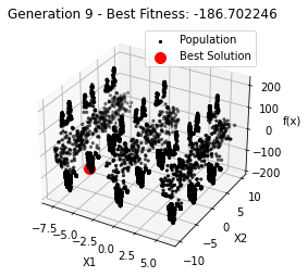
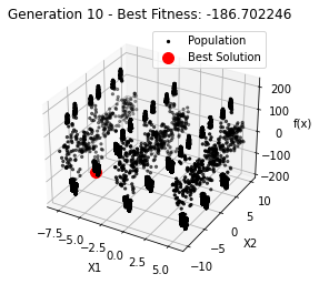
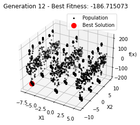
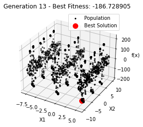
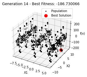
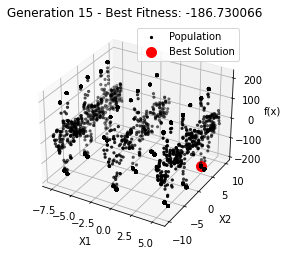
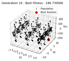
# 绘制每次迭代的三维分布图
fig = plt.figure() # 创建一个新的图形
ax = fig.add_subplot(111, projection='3d') # 创建一个三维的坐标系
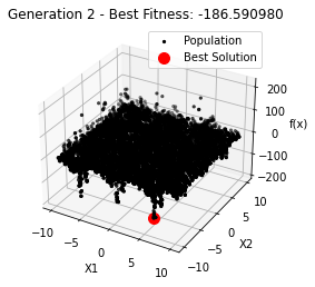
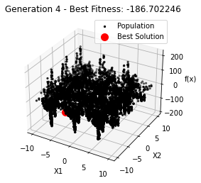
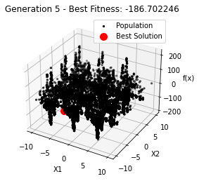
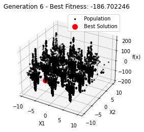
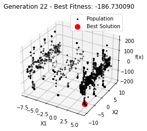
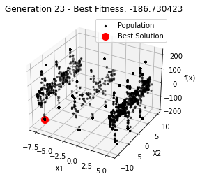
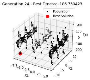
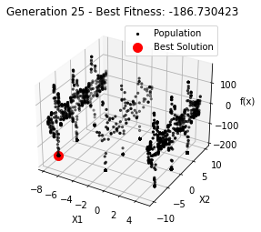
ax.scatter(population[:, 0], population[:, 1], fitness_values, color='black', marker='.', label='Population') # 绘制种群的分布图
ax.scatter(current_best_solution[0], current_best_solution[1], current_best_fitness, s=100, color='red', marker='o', label='Best Solution') # 绘制最佳解的分布图
# 设置坐标轴的标签
ax.set_xlabel('X1')
ax.set_ylabel('X2')
ax.set_zlabel('f(x)')
ax.set_title(f'Generation {
generation} - Best Fitness: {
current_best_fitness:.6f}')
ax.legend() # 显示图例
plt.show() # 显示图形
# 更新全局最佳解
if current_best_fitness < best_fitness: # 如果当前的最佳解的适应度值小于全局最佳解的适应度值
best_solution = current_best_solution
best_fitness = current_best_fitness
# 保存当前迭代步骤的信息
evolution_data.append({
'generation': generation,
'best_solution': best_solution,
'best_fitness': best_fitness
})
# 根据适应度值确定复制的数量并且形成繁殖池
reproduction_ratios = fitness_values / np.sum(fitness_values) # 计算每个个体的适应度值占总适应度值的比例
sorted_index_ratios = np.argsort(reproduction_ratios) # 对比例进行排序
half_length = len(sorted_index_ratios) // 2 # 选择后一半的个体
first_half_index = sorted_index_ratios[half_length:] # 选择后一半的个体的索引
new_half_population = population[first_half_index] # 选择后一半的个体
breeding_pool = np.concatenate((new_half_population, new_half_population)) # 将后一半的个体复制一份,形成繁殖池
# 选择父母
parents_1 = breeding_pool[:half_length]
parents_2 = breeding_pool[half_length:] # 先获取最后一半的父母
parents_2 = np.flip(parents_2, axis=0) # 再将父母的顺序反转
# 选择和交叉
parents_1, parents_2 = crossover(parents_1, parents_2, crossover_rate)
# 变异
parents_1, parents_2 = mutate(parents_1, parents_2, mutation_rate)
# 更新种群
population = np.vstack([parents_1, parents_2])
return best_solution, best_fitness, evolution_data
# 设置算法参数
population_size = 15000
num_generations = 40
mutation_rate = 0.08 # 变异率
crossover_rate = 0.2 # 交叉率
# 运行进化算法
best_solution, best_fitness, evolution_data = evolutionary_algorithm(population_size, num_generations, mutation_rate, crossover_rate)
# 输出结果
print("最小值:", best_fitness)
print("最优解:", best_solution)
# 输出每个迭代步骤的最佳适应度值
print("每个迭代步骤的最佳适应度值:")
for step in evolution_data:
print(f"Generation {
step['generation']}: {
step['best_fitness']}")
# 可视化函数曲面和最优解
x1_vals = np.linspace(-10, 10, 100)
x2_vals = np.linspace(-10, 10, 100)
X1, X2 = np.meshgrid(x1_vals, x2_vals)
Z = np.zeros_like(X1)
for i in range(Z.shape[0]):
for j in range(Z.shape[1]):
Z[i, j] = objective_function([X1[i, j], X2[i, j]])
fig = plt.figure()
ax = fig.add_subplot(111, projection='3d')
ax.plot_surface(X1, X2, Z, alpha=0.5, cmap='viridis')
ax.scatter(best_solution[0], best_solution[1], best_fitness, color='red', marker='o', label='Best Solution')
ax.set_xlabel('X1')
ax.set_ylabel('X2')
ax.set_zlabel('f(x)')
ax.set_title('Objective Function and Best Solution')
ax.legend()
# 绘制适应度值的变化曲线
evolution_df = pd.DataFrame(evolution_data)
plt.figure()
plt.plot(evolution_df['generation'], evolution_df['best_fitness'], label='Best Fitness')
plt.xlabel('Generation')
plt.ylabel('Fitness')
plt.title('Evolution of Fitness')
plt.legend()
plt.show()
5 附录
5.1 In[1] 输出


最小值: 1.0000002473000187
最优解: [0.78562713 0.7854951 ]
每个迭代步骤的最佳适应度值:
Generation 0: 1.0000153042180673
Generation 1: 1.0000153042180673
Generation 2: 1.0000153042180673
Generation 3: 1.0000136942409763
Generation 4: 1.0000136942409763
Generation 5: 1.0000136942409763
Generation 6: 1.0000136942409763
Generation 7: 1.0000100419077742
Generation 8: 1.000005565304546
Generation 9: 1.000002458099502
Generation 10: 1.0000022366988228
Generation 11: 1.0000007727585987
Generation 12: 1.0000007727585987
Generation 13: 1.0000007091648468
Generation 14: 1.0000007091648468
Generation 15: 1.0000004471760704
Generation 16: 1.0000004471760704
Generation 17: 1.0000004471760704
Generation 18: 1.0000004471760704
Generation 19: 1.0000002609708571
Generation 20: 1.0000002609708571
Generation 21: 1.0000002609708571
Generation 22: 1.0000002609708571
Generation 23: 1.0000002609708571
Generation 24: 1.0000002609708571
Generation 25: 1.0000002609708571
Generation 26: 1.0000002609708571
Generation 27: 1.0000002609708571
Generation 28: 1.0000002609708571
Generation 29: 1.0000002473000187
Generation 30: 1.0000002473000187
Generation 31: 1.0000002473000187
Generation 32: 1.0000002473000187
Generation 33: 1.0000002473000187
Generation 34: 1.0000002473000187
Generation 35: 1.0000002473000187
Generation 36: 1.0000002473000187
Generation 37: 1.0000002473000187
Generation 38: 1.0000002473000187
Generation 39: 1.0000002473000187
5.2 In[2] 输出


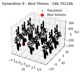


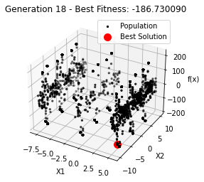
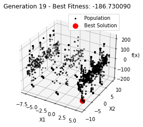
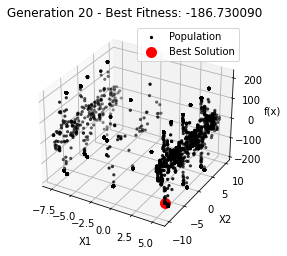
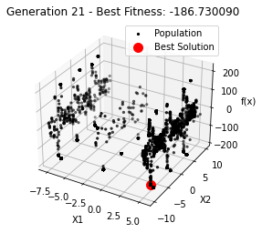
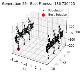


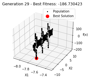
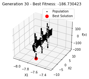
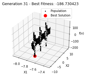

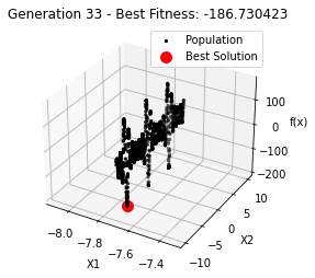
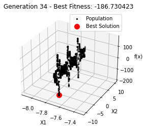

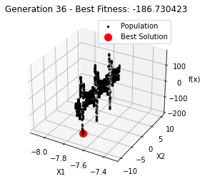

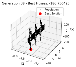

最小值: -186.73042323192567
最优解: [-7.70876845 -7.08354764]
每个迭代步骤的最佳适应度值:
Generation 0: -186.59098010602338
Generation 1: -186.59098010602338
Generation 2: -186.59098010602338
Generation 3: -186.59098010602338
Generation 4: -186.70224634663253
Generation 5: -186.70224634663253
Generation 6: -186.70224634663253
Generation 7: -186.70224634663253
Generation 8: -186.70224634663253
Generation 9: -186.70224634663253
Generation 10: -186.70224634663253
Generation 11: -186.71507272172664
Generation 12: -186.71507272172664
Generation 13: -186.7289048406221
Generation 14: -186.73006643615773
Generation 15: -186.73006643615773
Generation 16: -186.73006643615773
Generation 17: -186.73006643615773
Generation 18: -186.73009038074477
Generation 19: -186.73009038074477
Generation 20: -186.73009038074477
Generation 21: -186.73009038074477
Generation 22: -186.73009038074477
Generation 23: -186.73042323192567
Generation 24: -186.73042323192567
Generation 25: -186.73042323192567
Generation 26: -186.73042323192567
Generation 27: -186.73042323192567
Generation 28: -186.73042323192567
Generation 29: -186.73042323192567
Generation 30: -186.73042323192567
Generation 31: -186.73042323192567
Generation 32: -186.73042323192567
Generation 33: -186.73042323192567
Generation 34: -186.73042323192567
Generation 35: -186.73042323192567
Generation 36: -186.73042323192567
Generation 37: -186.73042323192567
Generation 38: -186.73042323192567
Generation 39: -186.73042323192567


![[二]rtmp服务器搭建](https://img-blog.csdnimg.cn/direct/12a45f3429ce42428d7424184844b645.png)