文章目录
机器学习算法实战案例系列
答疑&技术交流
技术要学会分享、交流,不建议闭门造车。一个人可以走的很快、一堆人可以走的更远。
本文完整代码、相关资料、技术交流&答疑,均可加我们的交流群获取,群友已超过2000人,添加时最好的备注方式为:来源+兴趣方向,方便找到志同道合的朋友。
方式①、微信搜索公众号:Python学习与数据挖掘,后台回复:加群
方式②、添加微信号:dkl88194,备注:来自CSDN + 技术交流
1 数据处理
1.1 导入库文件
import matplotlib.pyplot as plt

from sampen import sampen2  # sampen库用于计算样本熵

from vmdpy import VMD  # VMD分解库

from itertools import cycle

from sklearn.cluster import KMeans

from sklearn.metrics import r2_score, mean_squared_error, mean_absolute_error, mean_absolute_percentage_error

from sklearn.preprocessing import MinMaxScaler

from tensorflow.keras.models import Sequential

from tensorflow.keras.layers import Dense, Activation, Dropout, LSTM, GRU, Reshape, BatchNormalization

from tensorflow.keras.callbacks import ReduceLROnPlateau, EarlyStopping, ModelCheckpoint

from tensorflow.keras.optimizers import Adam

warnings.filterwarnings('ignore'))
plt.rcParams['font.sans-serif'] = ['SimHei']     # 显示中文

plt.rcParams['axes.unicode_minus'] = False  # 显示负号

plt.rcParams.update({
   'font.size':18})  #统一字体字号
1.2 导入数据集
实验数据集采用数据集8:新疆光伏风电数据集,数据集包括组件温度(℃) 、温度(°) 气压(hPa)、湿度(%)、总辐射(W/m2)、直射辐射(W/m2)、散射辐射(W/m2)、实际发电功率(mw)特征,时间间隔15min。对数据进行可视化:
from itertools import cycle

def visualize_data(data, row, col):

    cycol = cycle('bgrcmk')

    cols = list(data.columns)

    fig, axes = plt.subplots(row, col, figsize=(16, 4))

    if row == 1 and col == 1:  # 处理只有1行1列的情况

        axes = [axes]  # 转换为列表,方便统一处理

    for i, ax in enumerate(axes.flat):

        if i < len(cols):

            ax.plot(data.iloc[:,i], c=next(cycol))

            ax.set_title(cols[i])

            ax.axis('off')  # 如果数据列数小于子图数量,关闭多余的子图

    plt.subplots_adjust(hspace=0.6)

visualize_data(data_raw.iloc[:,1:], 2, 4)

单独查看部分功率数据,发现有较强的规律性。

1.3 缺失值分析
首先查看数据的信息,发现并没有缺失值

进一步统计缺失值
data_raw.isnull().sum()

2 VMD经验模态分解
2.1 VMD分解实验
使用VMD将目标信号分解成若干个模态,进一步可视化分解结果
def vmd_decompose(series=None, alpha=2000, tau=0, K=6, DC=0, init=1, tol=1e-7, draw=True):

    # 得到 VMD 分解后的各个分量、分解后的信号和频率

    imfs_vmd, imfs_hat, omega = VMD(series, alpha, tau, K, DC, init, tol)

    # 将 VMD 分解分量转换为 DataFrame, 并重命名

    df_vmd = pd.DataFrame(imfs_vmd.T)

    df_vmd.columns = ['imf'+str(i) for i in range(K)]
因为只是单变量预测,只选取实际发电功率(mw)数据进行实验。

查看分解后的数据:

这里我们验证一下分解效果,通过分解变量求和和实际功率值进行可视化比较,发现基本相同。
plt.figure(dpi=100,figsize=(14,5))

plt.plot(df_vmd.iloc[:96*10,:-1].sum(axis=1))

plt.plot(data_raw['实际发电功率(mw)'][:96*10])

plt.legend(['VMD分解求和','原始负荷'])

2.2 VMD-LSTM预测思路
这里利用VMD-LSTM进行预测的思路是通过VMD将原始功率分解为多个变量,然后将每个分解变量都进行预测,接着将预测的结果添加到历史数据中进行滚动预测,得到需要预测的步数,最后将每个分解变量的预测结果相加得到最终的预测结果。

3 构造训练数据
构造数据前先将数据变为数值类型
df_vmd = df_vmd.values
构造训练数据,也是真正预测未来的关键。首先设置预测的timesteps时间步、predict_steps预测的步长(预测的步长应该比总的预测步长小),length总的预测步长,参数可以根据需要更改。
通过前timesteps个数据预测后面predict_steps个数据,需要对数据集进行滚动划分(也就是前timesteps行的数据和后predict_steps行的数据训练,后面预测时就可通过timesteps行数据预测未来的predict_steps行数据)。这里需要注意的是,因为是多变量预测多变量,特征就是标签(例如,前5行[imf_0, imf_1, imf_2, imf_3, imf_4, imf_5]预测第6行[imf_0, imf_1, imf_2, imf_3, imf_4, imf_5],划分数据集时,就用前5行当做train_x,第6行作为train_y,此时的train_y有多列,而不是只有1列)。
# 整体的思路也就是,前面通过前timesteps个数据训练后面的predict_steps个未来数据

# 预测时取出前timesteps个数据预测未来的predict_steps个未来数据。

def create_dataset(datasetx, datasety=None, timesteps=96*7, predict_size=12):

    for each in range(len(datasetx) - timesteps - predict_size):

        x = datasetx[each:each + timesteps]

        # 判断是否是单变量分解还是多变量分解

        if datasety is not None:

            y = datasety[each + timesteps:each + timesteps + predict_size]

            y = datasetx[each + timesteps:each + timesteps + predict_size]

数据处理前,需要对数据进行归一化,按照上面的方法划分数据,这里返回划分的数据和归一化模型(变量和多变量的归一化不同,多变量归一化需要将X和Y分开归一化,不然会出现信息泄露的问题),此时的归一化相当于是单变量归一化,函数的定义如下:
def data_scaler(datax, datay=None, timesteps=36, predict_steps=6):

    scaler1 = MinMaxScaler(feature_range=(0, 1))

    datax = scaler1.fit_transform(datax)

    # 用前面的数据进行训练,留最后的数据进行预测

    if datay is not None:

        scaler2 = MinMaxScaler(feature_range=(0, 1))

        datay = scaler2.fit_transform(datay)

        trainx, trainy = create_dataset(datax, datay, timesteps, predict_steps)

        trainx = np.array(trainx)

        trainy = np.array(trainy)

        return trainx, trainy, scaler1, scaler2

        trainx, trainy = create_dataset(datax, timesteps=timesteps, predict_size=predict_steps)

        trainx = np.array(trainx)

        trainy = np.array(trainy)

        return trainx, trainy, scaler1, None
然后分解的数据进行划分和归一化。通过前7天的96*7行数据预测后一天的96个数据,需要对数据集进行滚动划分(也就是前96*7行的数据和后12行的数据训练,后面预测时就可通过96*7行数据测未来的12行数据,然后将12行预测值添加到历史数据中,历史数据变为96*7+12个,再取出后96*7行数据进行预测,得到12行预测值,滚动进行预测直到预测完成,注意此时的预测值是行而不是个)
trainx, trainy, scalerx, scalery = data_scaler(df_vmd, timesteps=timesteps, predict_steps=predict_steps)

4 LSTM模型训练
首先划分训练集、测试集、验证数据:
train_x = trainx[:int(trainx.shape[0] * 0.8)]

train_y = trainy[:int(trainy.shape[0] * 0.8)]

test_x = trainx[int(trainx.shape[0] * 0.8):]

test_y = trainy[int(trainy.shape[0] * 0.8):]

test_x.shape, test_y.shape, train_x.shape, train_y.shape
首先搭建模型的常规操作,然后使用训练数据trainx和trainy进行训练,进行50个epochs的训练,每个batch包含64个样本(建议使用GPU进行训练)。
def LSTM_model_train(trainx, trainy, valx, valy, timesteps, predict_steps):

    gpus = tf.config.experimental.list_physical_devices(device_type='GPU')

        tf.config.experimental.set_memory_growth(gpu, True)

    start_time = datetime.datetime.now()

    model.add(LSTM(128, input_shape=(timesteps, trainx.shape[2]), return_sequences=True))

    model.add(BatchNormalization())  # 添加BatchNormalization层

    model.add(Dropout(0.2))

    model.add(LSTM(64, return_sequences=False))

    model.add(Reshape((predict_steps, trainy.shape[2])))

    opt = Adam(learning_rate=0.001)

    model.compile(loss="mean_squared_error", optimizer=opt)

    es = EarlyStopping(monitor='val_loss', mode='min', verbose=1, patience=10)

    mc = ModelCheckpoint('best_model.h5', monitor='val_loss', mode='min', save_best_only=True)

    # 训练模型,这里我假设你有一个验证集(valx, valy)

    history = model.fit(trainx, trainy, validation_data=(valx, valy), epochs=50, batch_size=64, callbacks=[es, mc])

    loss_history = history.history['loss']

    end_time = datetime.datetime.now()

    running_time = end_time - start_time

    return model, loss_history, running_time
然后进行训练,将训练的模型、损失和训练时间保存。
model, loss_history, running_time = LSTM_model_train(train_x, train_y, test_x, test_y, timesteps, predict_steps)

model.save('emd_lstm_model.h5')
5 LSTM模型预测
5.1 分量预测
下面介绍文章中最重要,也是真正没有未来特征的情况下预测未来标签的方法。整体的思路也就是取出预测前96*6行数据预测未来的12行数据,然后见12行数据添加进历史数据,再预测12行数据,滚动预测。因为每次只能预测12行数据,但是我要预测96个数据,所以采用的就是循环预测的思路。每次预测的12行数据,添加到数据集中充当预测x,然后在预测新的12行y,再添加到预测x列表中,如此往复,最终预测出96行。(注意多变量预测多变量预测的是多列,预测单变量只有一列)
# #因为每次只能预测12个数据,但是我要预测96个数据,所以采用的就是循环预测的思路。

# #每次预测的12个数据,添加到数据集中充当预测x,然后在预测新的12个y,再添加到预测x列表中,如此往复,最终预测出96个点。

def predict_using_LSTM(model, data, timesteps, predict_steps, feature_num, length, scaler):

    predict_xlist = np.array(data).reshape(1, timesteps, feature_num)

    predict_y = np.array([]).reshape(0, feature_num)  # 初始化为空的二维数组

    print('predict_xlist', predict_xlist.shape)

    while len(predict_y) < length:

        # 从最新的predict_xlist取出timesteps个数据,预测新的predict_steps个数据

        predictx = predict_xlist[:,-timesteps:,:]
        print('predictx.shape', predictx.shape)

        lstm_predict = model.predict(predictx)

        print('lstm_predict.shape', lstm_predict.shape)

        # 将新预测出来的predict_steps个数据,加入predict_xlist列表,用于下次预测

        print('predict_xlist.shape', predict_xlist.shape)

        predict_xlist = np.concatenate((predict_xlist, lstm_predict), axis=1)

        print('predict_xlist.shape', predict_xlist.shape)

        # 预测的结果y,每次预测的12个数据,添加进去,直到预测length个为止

        lstm_predict = scaler.inverse_transform(lstm_predict.reshape(predict_steps, feature_num))

        predict_y = np.concatenate((predict_y, lstm_predict), axis=0)

        print('predict_y', predict_y.shape)
然后对数据进行预测,得到预测结果。
from tensorflow.keras.models import load_model

model = load_model('emd_lstm_model.h5')

pre_x = scalerx.fit_transform(df_vmd[-96*8:-96])

y_predict = predict_using_LSTM(model, pre_x, timesteps, predict_steps, feature_num, length, scalerx)
5.2 可视化
对预测的各分解变量和总的预测结果进行可视化。
for i in range(y_predict.shape[1]):

    fig, ax = plt.subplots(dpi=100, figsize=(14, 5))

    ax.plot(df_vmd[-96:, -i], markevery=5, label='IMF'+str(i)+'_true')

    ax.plot(y_predict[:, -i], markevery=5, label='IMF'+str(i)+'_predict')

    ax.legend(loc = 'upper right')

plt.figure(dpi=100, figsize=(14, 5))

plt.plot(np.sum(y_predict[:, :-1], axis=1), markevery=5, label = 'all_predict')

plt.plot(df_vmd[-96:,-1], markevery=5, label = 'all_true')

plt.legend(loc = 'upper right')


最后对预测结果计算误差。
def error_and_plot(y_true,y_predict):

    r2 = r2_score(y_true, y_predict)

    rmse = mean_squared_error(y_true, y_predict, squared=False)

    mae = mean_absolute_error(y_true, y_predict)

    mape = mean_absolute_percentage_error(y_true, y_predict)

    print("r2: %.2f\nrmse: %.2f\nmae: %.2f\nmape: %.2f" % (r2, rmse, mae, mape))

    cycol = cycle('bgrcmk')

    plt.figure(dpi=100, figsize=(14, 5))

    plt.plot(y_true, c=next(cycol), markevery=5)

    plt.plot(y_predict, c=next(cycol), markevery=5)

    plt.legend(['y_true', 'y_predict'])
error_and_plot(df_vmd[-96:,-1], np.sum(y_predict[:, :-1], axis=1) )