李沐机器学习系列2--- mlp

1 Introduction

LP中有一个很强的假设，输入和输出是线性关系，这一般是不符合事实的。
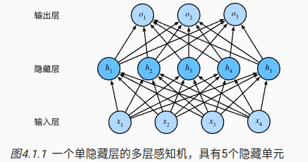
通过几何的方式去对信息进行理解和压缩是比较高效的，MLP可以表示成下面的形式。

1.1 从线性到非线性

$X\in R^{n\times d}$表示输入层，有n个样本，d个特征。
$H\in R^{n\times h}$表述隐藏层的输出，有h个输出；
$W^{(1)}\in R^{d\times h}$ 表示隐藏层的权重，$b^{(1)}\in R^{1\times h}$表示隐藏层的偏置
$W^{(2)}\in R^{h\times q}$和$b^{(2)}\in R^{1\times q}$分别是输出层的权重和偏置
$$\begin{array}{rl}H& =X\ast W^{(1)}+b^{(1)}\\ O& =H\ast W^{(2)}+b^{(2)}\end{array}$$
如果只是这样处理没有任何作用
$$O=X\ast W_1\ast W_2+b_1\ast W_2+b_2$$
关键还是需要一个非线性的激活函数，有了激活函数多层感知机就不会退化了。
$$\begin{array}{rl}H& =\sigma (X\ast W^{(1)}+b^{(1)})\\ O& =H\ast W^{(2)}+b^{(2)}\end{array}$$

1.2 激活函数

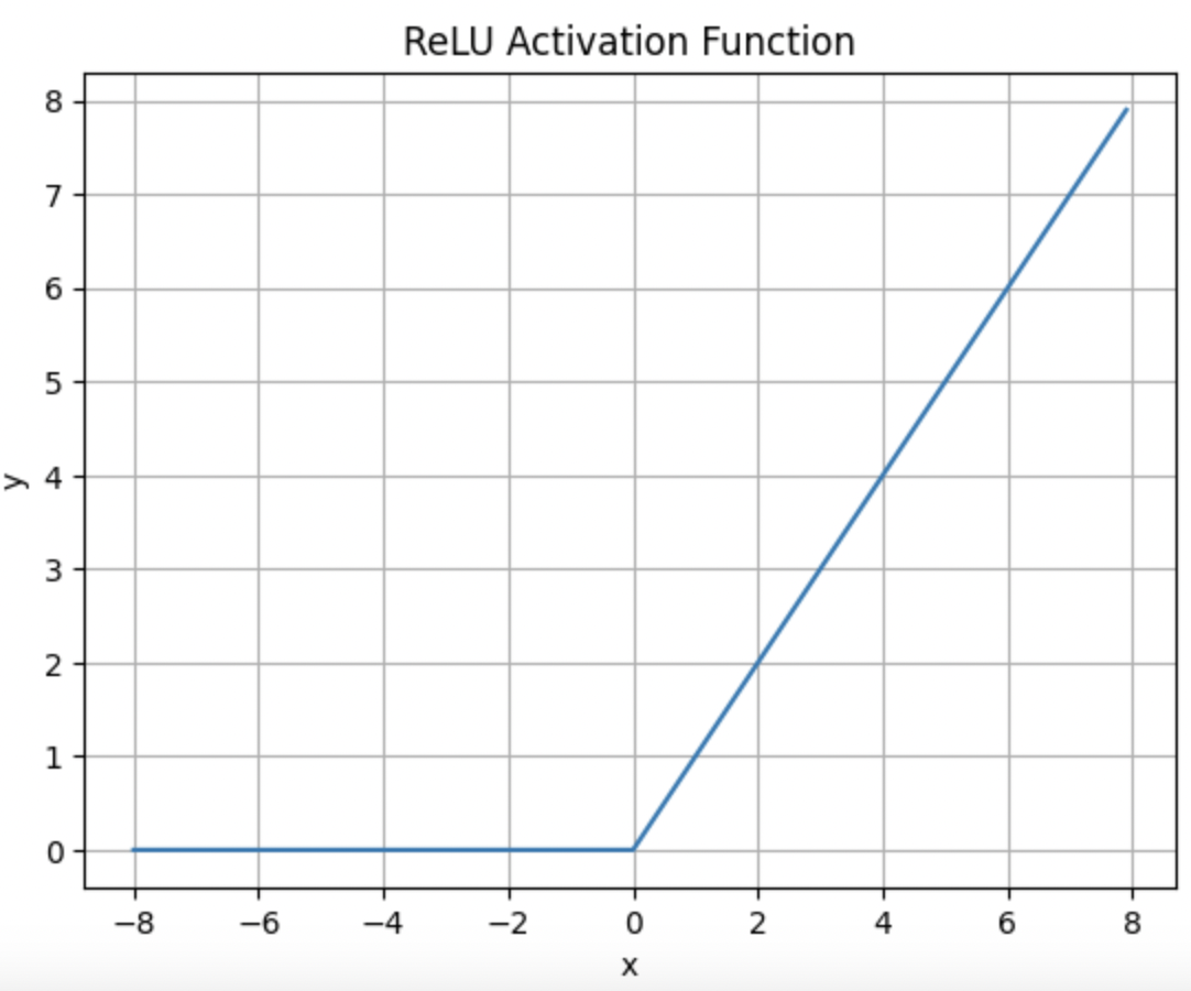
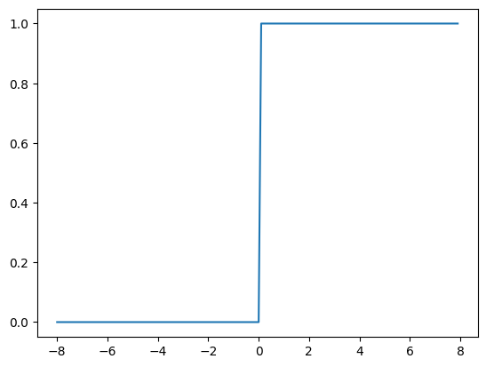
• RELU
  $$RELU(x)=max(0,x)$$

y.backward(torch.ones_like(x), retain_graph=True)
d2l.plot(x.detach(), x.grad, 'x', 'grad of relu', figsize=(5, 2.5))

y是一个向量，所以要指定torch.ones_like(x), 因为y是一个向量，所以需要retain_graph，防止计算图被销毁。

y.backward(torch.ones_like(x), retain_graph=True) # 保留计算图
plt.plot(x.detach(), x.grad)  

• sigmoid
  $$sigmoid(x)=\frac{1}{1+exp(-x)}$$

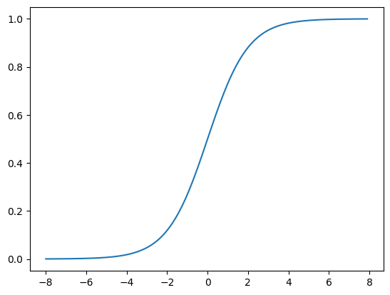
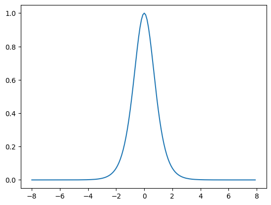
导数是

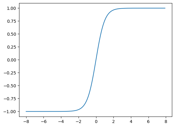
• tanh
  $$tanh(x)=\frac{1-exp(-2x)}{1+exp(-2x)}$$
  在0附近接近线性，
  
  

1.2 多层感知机

如果从零实现的话，需要自己定义个网络customNet

import torch
import torch.nn as nn
import torch.optim as optim
import matplotlib.pyplot as plt

import torchvision.transforms as transforms
from torch.utils.data import DataLoader

from torch import nn
from d2l import torch as d2l
batch_size = 256
transform = transforms.Compose([
    transforms.ToTensor(),
    transforms.Normalize((0.5,), (0.5,))
])

train_iter = torchvision.datasets.FashionMNIST(
    root='./data',
    train=True,
    download=True,
    transform=transform)
test_iter = torchvision.datasets.FashionMNIST(
    root='./data',
    train=False,
    download=True,
    transform=transform)
train_loader = DataLoader(train_iter, batch_size=batch_size, shuffle=True)
test_loader = DataLoader(test_iter, batch_size=batch_size, shuffle=False)


# Neural Network Class
class CustomNet(nn.Module):
    def __init__(self, num_inputs, num_hiddens, num_outputs):
        super(CustomNet, self).__init__()
        self.linear1 = nn.Linear(num_inputs, num_hiddens)
        self.linear2 = nn.Linear(num_hiddens, num_outputs)

    def forward(self, x):
        x = x.reshape((-1, num_inputs))
        H = torch.relu(self.linear1(x))
        return self.linear2(H)

# Network Parameters
num_inputs, num_hiddens, num_outputs = 784, 256, 10
net = CustomNet(num_inputs, num_hiddens, num_outputs)

# Loss Function and Optimizer
loss = nn.CrossEntropyLoss(reduction='mean')
updater = optim.SGD(net.parameters(), lr=0.1)

# Training Loop
num_epochs = 10
for epoch in range(num_epochs):
    total_loss = 0
    for x, y in train_loader:
        output = net(x)
        l = loss(output, y)
        updater.zero_grad()
        l.backward()
        updater.step()
        total_loss += l.item()
    print(f'Epoch {
     epoch + 1}, Average Loss: {
     total_loss / len(train_loader)}')

# Test the model
def test_model(net, test_loader):
    net.eval()  # Set the model to evaluation mode
    test_correct = 0
    total = 0
    with torch.no_grad():
        for x, y in test_loader:
            output = net(x)
            _, predicted = torch.max(output, 1)
            total += y.size(0)
            test_correct += (predicted == y).sum().item()
    return test_correct / total

accuracy = test_model(net, test_loader)
print(f'Test Accuracy: {
     accuracy:.2f}')

# Visualize one example
test_images, test_labels = next(iter(test_loader))
image, label = test_images[0], test_labels[0]

net.eval()
with torch.no_grad():
    output = net(image.unsqueeze(0))
    _, prediction = torch.max(output, 1)
    prediction = prediction.item()

# Display the image
plt.imshow(image.squeeze(), cmap='gray')
plt.title(f'Predicted: {
     prediction}, Actual: {
     label}')
plt.show()    

使用pytorch自带的网络定义工具

# Network Parameters
num_inputs, num_hiddens, num_outputs = 784, 256, 10

# Define the network using nn.Sequential
net = nn.Sequential(
    nn.Flatten(),
    nn.Linear(num_inputs, num_hiddens),
    nn.ReLU(),
    nn.Linear(num_hiddens, num_outputs)
)

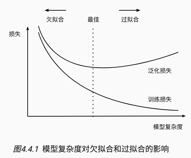
2 模型选择、欠拟合和过拟合

2.1 训练误差和泛化误差

2.1.1 统计学习理论

同名定理，训练误差收敛到泛化误差的速率。
独立同步分布假设，训练数据和测试数据都是从相同分布中独立提取出来。
有些假设符合独立同部分假设，人脸识别、语音识别和语言翻译任务；
有些假设不符合独立同分布，用大学生的人脸数据来检测养老院的老人。

2.1.2 模型复杂性

简单的模型和大量的数据，期待泛化误差和训练误差接近。需要更多训练迭代的模型比较复杂，较小训练迭代周期的不那么复杂。
影响泛化的因素：
1）可调参数的数量，模型往往更容易过拟合；
2）参数采用的值，权重的取值范围较大，更容易过拟合；
3）训练样本的数量；

2.1.3 验证集

需要通过验证集来进行模型筛选
训练和验证误差之间的泛化误差很小，欠拟合；

import math
import numpy as np
import torch
from torch import nn
from d2l import torch as d2l

max_degree = 20
n_train, n_test = 100, 100
true_w = np.zeros(max_degree)
true_w[0:4] = np.array([5, 1.2, -3.4, 5.6])

features = np.random.normal(size=(n_train + n_test, 1))
# print(features)
np.random.shuffle(features)
print(np.arange(max_degree).reshape(1, -1))
poly_features = np.power(features, np.arange(max_degree).reshape(1, -1))
print(poly_features)
for i in range(max_degree):
    poly_features[:, i] /= math.gamma(i + 1)

labels = np.dot(poly_features, true_w)
labels += np.random.normal(scale=0.1, size=labels.shape)

# 将pnumy array 转换成tensor
true_w, features, poly_features, labels = [torch.tensor(x, dtype=torch.float32)
                                          for x in [true_w, features, poly_features, labels]]
features[:2], poly_features[:2, :], labels[:2]

# 对模型进行训练
def evaluate_loss(net, data_iter, loss):
    metric = d2l.Accumulator(2)
    for x, y in data_iter:
        out = net(x)
        y = y.reshape(out.shape)
        l = loss(out, y)
        metric.add(l.sum(), l.numel())
    return metric[0]/metric[1]

def train(train_features, test_features, train_labels, test_labels,
          num_epochs=400):
    loss = nn.MSELoss(reduction='none')
    input_shape = train_features.shape[-1]
    net = nn.Sequential(nn.Linear(input_shape, 1, bias=False))
    batch_size = min(10, train_labels.shape[0])
    train_iter = d2l.load_array((train_features, train_labels.reshape(-1, 1)),
                               batch_size)
    test_iter = d2l.load_array((test_features, test_labels.reshape(-1, 1)),
                              batch_size, is_train=False)
    trainer = torch.optim.SGD(net.parameters(), lr=0.01)
    animator = d2l.Animator(xlabel='epoch', ylabel='loss', yscale='log',
                           xlim=[1, num_epochs], ylim=[1e-3,1e2],
                           legend=['train', 'test'])
    for epoch in range(num_epochs):
        d2l.train_epoch_ch3(net, train_iter, loss, trainer)
        if epoch == 0  or (epoch + 1) % 20 == 0:
            animator.add(epoch + 1, (evaluate_loss(net, train_iter, loss),
                                    evaluate_loss(net, test_iter, loss)))
    
    print('weight:', net[0].weight.data.numpy())

train(poly_features[:n_train, :4], poly_features[n_train:, :4],
     labels[:n_train], labels[n_train:])

3 权重衰减

在基础loss的基础上，增加对大权重的惩罚。

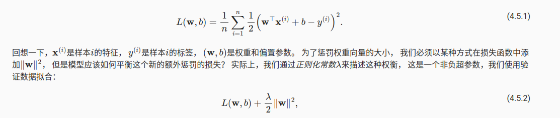
只要修改一下loss function,

def l2_penalty(w):
    return torch.sum(w.pow(2)) / 2
# 对模型进行训练
def train(lambd):
    w, b = init_params()
    net, loss = lambda X: d2l.linreg(X, w, b), d2l.squared_loss
    num_epochs, lr = 100, 0.003
    animator = d2l.Animator(xlabel='epochs', ylabel='loss', yscale='log',
                            xlim=[5, num_epochs], legend=['train', 'test'])
    for epoch in range(num_epochs):
        for X, y in train_iter:
            # 增加了L2范数惩罚项，
            # 广播机制使l2_penalty(w)成为一个长度为batch_size的向量
            l = loss(net(X), y) + lambd * l2_penalty(w)
            l.sum().backward()
            d2l.sgd([w, b], lr, batch_size)
        if (epoch + 1) % 5 == 0:
            animator.add(epoch + 1, (d2l.evaluate_loss(net, train_iter, loss),
                                     d2l.evaluate_loss(net, test_iter, loss)))
    print('w的L2范数是：', torch.norm(w).item())

在pytorch上可以同步衰减权重和参数

def train_concise(wd):
    net = nn.Sequential(nn.Linear(num_inputs, 1))
    for param in net.parameters():
        param.data.normal_()
    loss = nn.MSELoss(reduction='none')
    num_epochs, lr = 100, 0.003
    # 偏置参数没有衰减
    trainer = torch.optim.SGD([
        {
   "params":net[0].weight,'weight_decay': wd},
        {
   "params":net[0].bias}], lr=lr)
    animator = d2l.Animator(xlabel='epochs', ylabel='loss', yscale='log',
                            xlim=[5, num_epochs], legend=['train', 'test'])
    for epoch in range(num_epochs):
        for X, y in train_iter:
            trainer.zero_grad()
            l = loss(net(X), y)
            l.mean().backward()
            trainer.step()
        if (epoch + 1) % 5 == 0:
            animator.add(epoch + 1,
                         (d2l.evaluate_loss(net, train_iter, loss),
                          d2l.evaluate_loss(net, test_iter, loss)))
    print('w的L2范数：', net[0].weight.norm().item())

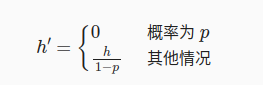
4 dropout

随机去掉一些节点，

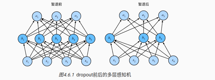
标准暂退法

这里因为dropout层的参数被mask了，输出为0，在反向传播的时候，更新的数值很小

def dropout_layer(X, dropout):
    assert 0 <= dropout <= 1
    # 在本情况中，所有元素都被丢弃
    if dropout == 1:
        return torch.zeros_like(X)
    # 在本情况中，所有元素都被保留
    if dropout == 0:
        return X
    mask = (torch.rand(X.shape) > dropout).float()
    return mask * X / (1.0 - dropout)
    
dropout1, dropout2 = 0.2, 0.5

class Net(nn.Module):
    def __init__(self, num_inputs, num_outputs, num_hiddens1, num_hiddens2,
                 is_training = True):
        super(Net, self).__init__()
        self.num_inputs = num_inputs
        self.training = is_training
        self.lin1 = nn.Linear(num_inputs, num_hiddens1)
        self.lin2 = nn.Linear(num_hiddens1, num_hiddens2)
        self.lin3 = nn.Linear(num_hiddens2, num_outputs)
        self.relu = nn.ReLU()

    def forward(self, X):
        H1 = self.relu(self.lin1(X.reshape((-1, self.num_inputs))))
        # 只有在训练模型时才使用dropout
        if self.training == True:
            # 在第一个全连接层之后添加一个dropout层
            H1 = dropout_layer(H1, dropout1)
        H2 = self.relu(self.lin2(H1))
        if self.training == True:
            # 在第二个全连接层之后添加一个dropout层
            H2 = dropout_layer(H2, dropout2)
        out = self.lin3(H2)
        return out


net = Net(num_inputs, num_outputs, num_hiddens1, num_hiddens2)

在pytorch后面，添加一个mask的dropout层就可以实现

net = nn.Sequential(nn.Flatten(),
        nn.Linear(784, 256),
        nn.ReLU(),
        # 在第一个全连接层之后添加一个dropout层
        nn.Dropout(dropout1),
        nn.Linear(256, 256),
        nn.ReLU(),
        # 在第二个全连接层之后添加一个dropout层
        nn.Dropout(dropout2),
        nn.Linear(256, 10))

def init_weights(m):
    if type(m) == nn.Linear:
        nn.init.normal_(m.weight, std=0.01)

net.apply(init_weights);

5 参数初始化

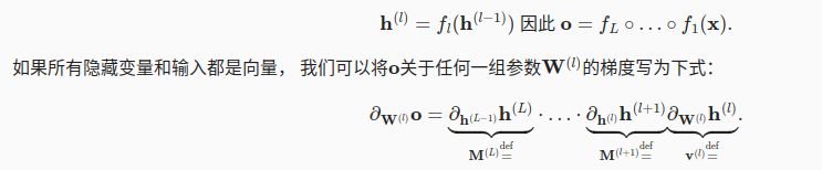
5.1 梯度爆炸

如果模型有L层，那么每层之间的参数进行更新的时候，梯度满足下面的关系。因为参数的grad有乘积关系，容易出现梯度爆炸和梯度消失。

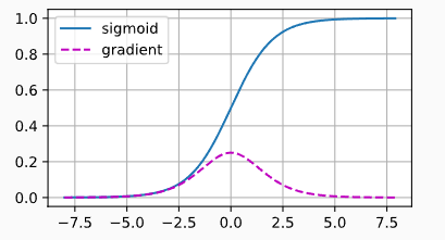
sigmoid函数的梯度消失
当参数很大或者很小，gradient都很小，经过多次传递之后，直接梯度消失了

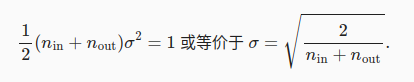
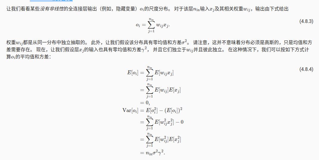
5.2 xavier 参数初始化

保证梯度的方差不变

6 分布和偏移