TensorFlow的实战（详细代码）

1 TensorFlow基础

　　1.1 TensorFlow概要

• TensorFlow使用数据流式图规划计算流程，它可以将计算映射到不同的硬件和操作系统平台。

　　1.2 TensorFlow编程模型简介

• TensorFlow中的计算可表示为一个有向图(计算图)，其中每个运算操作为一个节点，每个节点可有任意多个输入和输出；
• 在计算图的边中流动(flow)的数据被称为张量(tensor)，tensor在计算图中flow，故命名为TensorFlow；
• Session是用户使用TensorFlow的交互式接口，可通过Session的Extend方法添加新的节点和边；
• 反复执行计算图时一般的tensor不会被持续保留，Variable中的数据tensor会被保存。

2 TensorFlow和其他深度学习框架的对比

3 TensorFlow第一步

　　3.1 TensorFlow的编译及安装

　　3.2 TensorFlow实现Softmax Regression识别手写数字

• 载入MNIST数据集

  from tensorflow.examples.tutorials.mnist import input_data
  import tensorflow as tf
  mnist = input_data.read_data_sets("Mnist_data/", one_hot=True)

• 创建placeholder用以输入数据

  x = tf.placeholder(tf.float32, [None, 784])
  y_ = tf.placeholder(tf.float32, [None, 784])
  #None代表不限条数的输入

• 给模型中的weights和biases创建Variable对象，以存储模型参数(其他的tensor将不保存)

  W = tf.Variable(tf.zeros([784, 10]))
  b = tf.Variable(tf.zeros([10]))

• 构建计算公式

  y = softmax(Wx + b)

• 定义Loss，确定优化器

  cross_entropy = tf.reduce_mean(-tf.reduce_sum(y_ * tf.log(y), reduction_indices=[1]))
  train_step = tf.train.GradientDescentOptimizer(0.5).minimize(cross_entropy)

• 初始化变量，执行计算

  tf.global_variables_initializer().run()
  
  for i in range(1000):
      batch_xs, batch_ys = mnist.train.next_batch(100)
      train_step.run({x: batch_xs, y_: batch_ys})

4 TensorFlow实现自编码器及多层感知机

　　4.1 自编码器简介

• 自编码器，即可以使用自身的高阶特征编码自己；
• 特征的稀疏表达：使用少量的基本特征组合拼装得到更高层抽象的特征；
• 为防止简单的映射，加入几种限制：1. 让中间隐含层节点数量小于输入、输出节点数量，相当于降维  2. 给输入数据加入噪声

　　4.2 TensorFlow实现自编码器

• 用到xavier参数初始化方法

  def xavier_init(fan_in, fan_out, constant = 1):
      low = - constant * np.sqrt(6.0 / (fan_in + fan_out))
      high = constant * np.sqrt(6.0 / (fan_in + fan_out))
      return tf.random_uniform((fan_in, fan_out),
                                              minval=;ow, maxval=high,
                                              dtype=tf.float32)

• 参数初始化函数_initial_weights（创建一个名为all_weights的字典dict，将w1、b1、w2、b2全部存入其中）

  

  def _initialize_weights(self):
      all_weights = dict()
      all_weights['w1'] = tf.Variable(xavier_init(self.n_input, self.n_hidden))
      all_weights['b1'] = tf.Variable(tf.zeros([self.n_hidden], dtype=tf.float32))
      all_weights['w2'] = tf.Variable(xavier_init([self.n_hidden,
                                                   self.n_input], dtype=tf.float32))
      all_weights['b2'] = tf.Variable(tf.zeros([self.n_input],
                                                dtype=tf.float32))
      return all_weights

  

　　4.3 多层感知机简介

• Dropout是在训练时将神经网络某一层的输出节点数据随机丢弃一部分(训练时小于1,预测时等于1),这等于创造出了很多新的随机样本,也算是一种bagging
• Dropout是在训练时将神经网络某一层的输出节点数据随机丢弃一部分(训练时小于1,预测时等于1),这等于创造出了很多新的随机样本,也算是一种bagging

　　　　1. 单侧抑制

　　　　2. 相对宽阔的兴奋边界

　　　　3. 稀疏激活性

　　4.4 TensorFlow实现多层感知机

• ReLU层的权重可以用截断正态分布进行初始化,偏置可以用一些小的非零值来初始化以避免dead neuron.Sigmoid层的权重和偏置则都初始化为0即可
• 使用ReLU作为隐藏层,并添加dropout,就实现了多层感知机

5 TensorFlow实现卷积神经网络

　　5.1 卷积神经网络简介

• CNN最初是为解决图像识别问题设计，现在也可用于时间序列信号如音频、文本；
• CNN要点：局部连接、权值共享、池化层降采样

　　　　1. 局部连接和权值共享降低了参数量，减轻过拟合

　　　　2. 池化层降采样进一步降低输出参数量

• 只要卷积核数量足够多，能提取出各种方向的边或各种形态的点，就可以让采卷积层抽象出有效而丰富的高阶特征；
• CNN参数量只与卷积核尺寸和个数有关

　　5.2 TensorFlow实现简单的卷积网络

• 首先载入MNIST数据集
• 这个CNN会有很多权重和偏置需要创建，因此先定义初始化函数以便后续重复使用

  

  def weight_variable(shape):
      initial = tf.truncated_normal(shape, stddev=0.1)
      return tf.Variable(initial)
  
  def bias_variable(shape):
      initial = tf.constant(0.1, shape=shape)
      return tf.Variable(initial)

  

• 卷积层、池化层也需重复使用，这里分别定义创建函数

  def conv2d(x, W):
      return tf.nn.conv2d(x, W, strides=[1, 1, 1, 1], padding='SAME')
  
  def max_pool_2x2(x):
      return tf.nn.max_pool(x, ksize=[1, 2, 2, 1], strides=[1, 2, 2, 1], padding='SAME')

• 定义输入：x是特征，y_是真实的label

  x = tf.placeholder(tf.float32, [None, 784])
  y_ = tf.placeholder(tf.float32, [NOne, 10])
  x_image = tf.reshape(x, [-1, 28, 28, 1])

• 第一个卷积层

  W_conv1 = weight_variable([5, 5, 1, 32])
  b_conv1 = bias_variable([32])
  h_conv1 = tf.nn.relu(conv2d(x_image, W_conv1) + b_conv1)
  h_pool1 = max_pool_2x2(h_conv1)

• 第二个卷积层

  W_conv2 = weight_variable([5, 5, 32, 64])
  b_conv2 = bias_variable([64])
  h_conv2 = tf.nn.relu(conv2d(h_pool1, W_conv2) + b_conv2)
  h_pool2 = max_pool_2x2(h_conv2)

• 第一个全连接层，后接dropout

  W_fc1 = weight_variable([7*7*64, 1024])
  b_fc1 = bias_variable([1024])
  h_pool2_flat = tf.reshape(h_pool2, [-1, 7*7*64])
  h_fc1 = tf.nn.relu(tf.matmul(h_pool2_flat, W_fc1) + b_fc1)
  
  keep_prob = tf.placeholder(tf.float32)
  h_fc1_drop = tf.nn.dropout(h_fc1, keep_prob)

• 第二个全连接层，后接softmax

  W_fc2 = weight_variable([1024, 10])
  b_fc2 = bias_variable([10])
  y_conv = tf.nn.softmax(tf.matmul(h_fc1_drop, W_fc2) + b_fc2)

• 定义损失函数cross entropy，优化器使用Adam，学习速率1e-4

  cross_entropy = tf.reduce_mean(-tf.reduce_sum(y_ * tf.log(y_conv), reductioin_indices=[1]))
  train_step = tf.train.AdamOptimizer(1e-4).minimize(cross_entropy)

• inference完成后，开始训练

  tf.global_variables_initializer().run()
  for i in range(20000):
      batch = mnist.train.next_batch(50)
      train_step.run(feed_dict={x: batch[0], y_: batch[1], keep_prob: 0.5})

　　5.3 TensorFlow实现进阶的卷积网络

• 定义初始化weight函数

　　　　1. 这里给weight加一个L2的loss，相当于做了一个L2正则化处理

　　　　2. tf.multiply让L2 loss与wl(weight loss)相乘，即用wl控制L2 loss的大小(tf.mutmul矩阵乘法、tf.multiply点乘）

　　　　3. 使用tf.add_to_collection把weight loss同意存到名为“losses"的列表中（tf.get_colletion("name")获取列表）

def variable_with_weight_loss(shape, stddev, wl):
    var = tf.Variable(tf.truncated_normal(shape, stddev=stddev))
    if wl is not None:
        weight_loss = tf.multiply(tf.nn.l2_loss(var), wl, name='weight_loss')
        tf.add_to_collection('losses', weight_loss)
    return var

• 第一个卷积层

  weight1 = variable_with_weight_loss(shape=[5, 5, 3, 64], stddev=5e-2, wl=0.0)
  kernel1 = tf.nn.conv2d(image_input, weight1, [1, 1, 1, 1], padding='SAME')
  bias = tf.Variable(tf.constant(0.0, shape[64]))
  conv1 = tf.nn.relu(tf.nn.bias_add(kernel1, bias1))
  pool1 = tf.nn.max_pool(conv1, ksize=[1, 3, 3, 1], strides=[1, 2, 2, 1], padding='SAME')
  norm1 = tf.nn.lrn(pool1, 4, bias=1.0, alpha=0.001 / 9.0, beta=0.75)

• 数据增强(Data Augmentation)：对图片进行翻转、随机剪切，制造更多样本

6 TensorFLow实现经典卷积神经网络

　　6.1 TensorFlow实现AlexNet

• 使用ReLu，在较深的网络中效果好于Sigmoid，解决了Sigmoid在深层网络中梯度弥散问题
• 使用Dropout，避免模型过拟合
• 提出LRN
• 使用CUDA加速训练
• 数据增强

  def inference(images):
      parameters = []
      
      with tf.nn.name_scope('conv1') as scope:
          kernel = tf.Variable(tf.truncated_normal([11, 11, 3, 64], 
                                       dtype=tf.float32, stddev=1e-1), name='weights')
          conv = tf.nn.con2d(images, kernel, [1, 4, 4, 1], padding='SAME')
          biases = tf.Variable(tf.constant(0.0, shape=[64], dtype=tf.float32),
                                       trainable=True, name='biases')
          bias = tf.nn.bias_add(conv, biases)
          conv1 = tf.nn.relu(bias, name=scope)
          print_activation(conv1)
          parameters += [kernel, biases]
  
          lrn1 = tf.nn.lrn(conv1, 4, bias=1.0, alpha=0.001/9, beta=0.75, name='lrn1')
          pool1 = tf.nn.max_pool(lrn1, ksize=[1, 3, 3, 1], strides=[1, 2, 2, 1],
                                              padding='VALID', name='pool1')
          print_activations(pool1)

  6.2 TensorFlow实现VGGNet

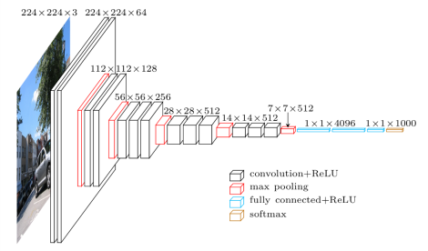
•  卷积核都为3x3，池化层都为2x2
• 3个3x3卷积层串联相当于1个7x7卷积层(感受野相同)，参数为后者55%
• 使用数据增强
• vgg16包含很多层，先创建函数conv_op、fc_op和mpool_op

  def conv_op(input_op, name, kh, kw, n_out, dh, dw, p):
      n_in = input_op.get_shape()[-1].value
      
      with tf.name_scope(name) as scope:
          kernel = tf.get_variable(scope+"w", shape=[kh, kw, n_in, n_out], dtype=tf.float32,
                                              initializer=tf.contrib.layers.xavier_initializer_conv2d())
          conv = tf.nn.conv2d(input_op, kernel, (1, dh, dw, 1), padding='SAME')
          bias_init_val = tf.constant(0.0, shape=[n_out], dtype=tf.float32)
          biases = tf.Variable(bias_init_val, trainable=True, name='b')
          z = tf.nn.bias_add(conv, biases)
          activation = tf.nn.relu(z, name=scope)
          p += [kernel, biases]
          return activation
  
  def fc_op(input_op, name, n_out, p):
      n_in = input_op.get_shape()[-1].value
  
      with tf.name_scope(name) as scope:
          kernel = tf.get_variable(scope+"w", shape=[n_in, n_out], dtype=tf.float32,
                                              initializer=tf.contrib.layers.xavier_initializer())
          biases = tf.Variable(tf.constant(0.1, shape=[n_out], dtype=tf.float32), name='b')
          activation = tf.nn.relu_layer(input_op, kernel, biases, name=scope)
          p += [kernel, biases]
          return activation
  
  def mpool_op(input_op, name, kh, kw, dh, dw):
      return tf.nn.max_pool(input_op, ksize=[1, kh, kw, 1], strides=[1, dh, dw, 1],
                                       padding='SAME', name=name)
  

•  完成创建函数，开始构建VGG16网络结构

  def inference_op(input_op, keep_prob):
      p = []
      
      conv1_1 = conv_op(input_op, name="conv1_1", kh=3, kw=3, n_out=64, dh=1, dw=1,
                                      p=p)
      conv1_2 = conv_op(conv1_1, name="conv1_2", kh=3,pool1",w=3, n_out=64, dh=1, dw=1,
                                      p=p)
      pool1 = mpool_op(conv1_2, name="pool1", kh=2, kw=2, dw=2, dh=2)
      ...

　　6.3 TensorFlow实现Google Inception Net

•  Inception V1去除最后的全连接层，用全局平均池化层代替。（模型训练更快且减轻了过拟合）
• 1x1卷积可以跨通道组织信息，提高网络表达能力，且可以对输出通道升维、降维
• 1x1卷积的性价比很高，用很小的计算量就能增加一层特征变化和非线性化
• 1x1卷积可很自然地把相关性很高的、在同一个空间位置但是不同通道的特征连接在一起
• 靠后的Inception Module中大面积的卷积核占比更多，以捕捉更高阶的抽象特征
• 用到辅助分类节点(auxiliary classifiers)，在Inception Net中间一层的输出用作分类，并按一个较小权重(0.3)加到最终分类结果中
• Inception V2提出了Batch Normalization
• 定义inception_v3_arg_scope用来生成网络中经常用到的函数的默认参数

  def inception_v3_arg_scope(weight_decay=0.00004, stddev=0.1,
                                              batch_norm_var_collectioin='moving_vars'):
      batch_norm_params = {
          'decay': 0.9997,
          'epsilon': 0.001,
          'updates_collections': tf.GraphKeys.UPDATE_OPS,
          'variables_collections': {
              'beta': None,
              'gamma': None,
              'moving_mean': [batch_norm_var_collectioin],
              'moving_variance': [batch_norm_var_collection],
          }
      }
  with slim.arg_scope([slim.conv2d, slim.fully_connected],
                                  weights_regularizer=slim.l2_regularizer(weight_decay)):
      with slim.arg_scope([slim.conv2d],
                                      weights_initializer=tf.truncated_normal_initializer(stddev=stddev),
                                      activation_fn=tf.nn.relu,
                                      normalizer_fn=slim.batch_norm,
                                      normalizer_params=batch_norm_params) as sc:
          return sc

• 定义inception_v3_base用来生成Inception V3网络的卷积部分

  def inception_v3_base(inputs, scope=None):
      end_points = {}
      with tf.variable_scope(scope, 'InceptionV3', [inputs]):
          #前面的卷积层
          with slim.arg_scope([slim.conv2d, slim.max_pool2d, slim.avg_pool2d],
                                          stride=1, padding='VALID'):
              net = slim.conv2d(inputs, 32, [3, 3], stride=2, scope='Conv2d_1a_3x3')
              net = slim.conv2d(net, 32, [3, 3], scope='Conv2d_2a_3x3')
              ...
          #接着是三个Inception
          #inception 1
          with slim.arg_scope([slim.conv2d, slim.max_pool2d, slim.avg_pool2d],
                                          stride=1, padding='SAME'):
              
                #inception 1中的第一个inception module
               with tf.variable_scope('Mixed_5b'):
                  with tf.variable_scope('Branch_0'):
                      branch_0 = slim.conv2d(net, 64, [1, 1], scope='Conv2d_0a_1x1')
                  with tf.variable_scope('Branch_1'):
                      branch_1 = slim.conv2d(net, 48, [1, 1], scope='Conv2d_0a_1x1')
                      branch_1 = slim.conv2d(branch_1, 64, [5, 5], scope='Conv2d_0b_5x5')    
              ...

  6.4 TensorFlow实现ResNet

• ResNet的残差学习单元(Residual Unit)不再学习一个完整的输出H(x),而是学习残差H(x)-x.ResNet有很多支线将输入直接连到后面的层,使得后面的层可以直接学习残差,这种结构被称为shortcut
• 两层的残差学习单元包含两个相同输出通道数的3x3卷积,三层的残差学习单元则是1x1卷积,3x3卷积,1x1卷积,并且先降维再升维