参考文章:
在过去的几年里,关于卷积神经网络(CNN)的讨论很多,特别是因为它们彻底改变了计算机视觉领域。在这篇文章中,我们将建立在神经网络的基本背景知识的基础上,探索什么是 CNN,了解它们是如何工作的,并在 Python 中从头开始(仅使用 numpy)构建一个真正的 CNN。
一、目的
CNN 的一个经典用例是执行图像分类,例如查看宠物的图像并确定它是猫还是狗。这是一项看似简单的任务——为什么不直接使用普通的神经网络呢?
问得好。
原因1:图像很大
如今,用于计算机视觉问题的图像通常是 224x224 或更大。想象一下,构建一个神经网络来处理 224x224 彩色图像:包括图像中的 3 个颜色通道 (RGB),结果是 224 x 224 x 3 = 150,528 个输入特征!在这样的网络中,一个典型的隐藏层可能有 1024 个节点,因此我们必须单独训练第一层的 150,528 x 1024 = 150+ 百万权重。我们的网络将是巨大的,几乎不可能训练。
我们也不是需要那么多砝码。图像的好处在于,我们知道像素在其邻居的上下文中最有用。图像中的对象由小的局部特征组成,例如眼睛的圆形虹膜或一张纸的方角。第一个隐藏层中的每个节点查看每个像素似乎不是很浪费吗?
原因 2:物体位置可能会发生变化
如果你训练了一个网络来检测狗,你会希望它能够检测一只狗,而不管它出现在图像中的哪个位置。想象一下,训练一个网络,该网络在某个狗图像上运行良好,然后向它提供同一图像的略微偏移版本。狗不会激活相同的神经元,因此网络的反应会完全不同!
我们很快就会看到CNN如何帮助我们缓解这些问题。
二. 数据集
在这篇文章中,我们将解决计算机视觉的“Hello, World!”:MNIST手写数字分类问题。这很简单:给定一张图像,将其归类为数字。
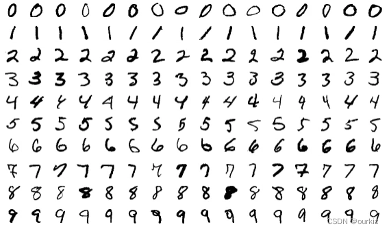
来自 MNIST 数据集的示例图像
MNIST数据集下载地址:点击下载
MNIST 数据集中的每张图像都是 28x28 的,并包含一个居中的灰度数字。
说实话,一个普通的神经网络实际上可以很好地解决这个问题。您可以将每个图像视为一个 28 x 28 = 784 维的矢量,将其馈送到 784 度的输入层,堆叠一些隐藏层,最后形成一个包含 10 个节点的输出层,每个数字 1 个。
这只会起作用,因为 MNIST 数据集包含居中的小图像,因此我们不会遇到上述大小或移动问题。然而,请记住,在这篇文章的整个过程中,大多数现实世界的图像分类问题并不是那么容易。
足够的积累。让我们进入CNN吧!
三. 卷积
什么是卷积神经网络?
它们基本上只是使用卷积层的神经网络,也就是Conv 层,它基于卷积(将被卷积对象的值对y轴翻转,右移,与卷积对象进行上下相乘求和所得到的一个结果)的数学运算。Conv 层由一组过滤器组成,您可以将其视为数字的 2D 矩阵。下面是一个 3x3 的过滤器示例:

我们可以使用输入图像和过滤器通过将过滤器与输入图像进行卷积来生成输出图像。这包括
- 将滤镜叠加在图像顶部的某个位置。
- 在过滤器中的值与其在图像中的相应值之间执行元素乘法。
- 对所有元素进行求和,此总和是输出图像中目标像素的输出值。
- 对所有位置重复上述步骤。
旁注:从技术上讲,我们(以及许多CNN实现)实际上在这里使用互相关而不是卷积,但它们几乎做同样的事情。我不会在这篇文章中讨论其中的区别,因为它并不那么重要,但如果您好奇,请随时查找。
这个 4 步描述有点抽象,所以让我们举个例子。考虑这个小的 4x4 灰度图像和这个 3x3 过滤器:

4x4 图像(左)和 3x3 滤镜(右)
图像中的数字表示像素强度,其中 0 表示黑色,255 表示白色。我们将对输入图像和过滤器进行卷积,以生成 2x2 的输出图像:

2x2 输出图像
首先,让我们在图像的左上角叠加我们的过滤器:

第 1 步:将过滤器(右)叠加在图像(左)的顶部
接下来,我们在重叠的图像值和过滤器值之间执行元素乘法。以下是结果,从左上角开始,向右走,然后向下走:
| 图像值 | 过滤器值 | 结果 |
|---|---|---|
| 0 | -1 | 0 |
| 50 | 0 | 0 |
| 0 | 1 | 0 |
| 0 | -2 | 0 |
| 80 | 0 | 0 |
| 31 | 2 | 62 |
| 33 | -1 | -33 |
| 90 | 0 | 0 |
| 0 | 1 | 0 |
第 2 步:执行元素乘法。
接下来,我们对所有结果进行相加。这很简单: 62−33=29
最后,我们将结果放在输出图像的目标像素中。由于我们的过滤器覆盖在输入图像的左上角,因此我们的目标像素是输出图像的左上角像素:

我们将如此重复对所有像素做同样的操作,如下:

3.1 这有什么用?
让我们缩小一秒钟,在更高的层面上看到这一点。使用滤镜对图像进行卷积有什么作用?我们可以从使用我们一直在使用的示例 3x3 滤波器开始,它通常称为垂直 Sobel 滤波器:
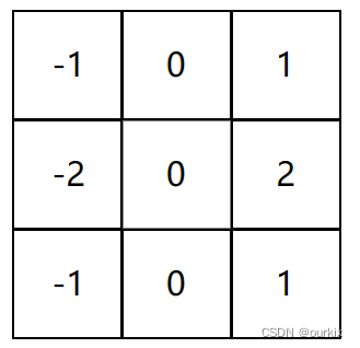
立式 Sobel 过滤器
下面是垂直 Sobel 过滤器的示例:

使用垂直 Sobel 滤波器卷积的图像
同样,还有一个水平 Sobel 过滤器:

使用水平 Sobel 滤波器卷积的图像
看看发生了什么?Sobel 滤波器是边缘检测器。垂直 Sobel 滤波器检测垂直边缘,水平 Sobel 滤波器检测水平边缘。输出图像现在很容易解释:输出图像中的明亮像素(具有高值的像素)表明原始图像周围有很强的边缘。
您能理解为什么边缘检测图像可能比原始图像更有用吗?回想一下我们的MNIST手写数字分类问题。例如,在MNIST上训练的CNN可能会通过使用边缘检测过滤器并检查图像中心附近的两个突出的垂直边缘来查找数字1。一般来说,卷积可以帮助我们寻找特定的局部图像特征(如边缘),以便我们稍后在网络中使用。
3.2 填充
还记得之前使用 4x4 滤波器对 3x3 输入图像进行卷积以生成 2x2 输出图像吗?通常,我们更希望输出图像的大小与输入图像的大小相同。为此,我们在图像周围添加零,以便我们可以在更多位置叠加滤镜。3x3 滤镜需要 1 像素的填充:

这称为“相同”填充,因为输入和输出具有相同的尺寸。不使用任何填充,这是我们一直在做的,,有时被称为“有效”填充。
3.3 转换层
现在我们知道了图像卷积的工作原理以及它为什么有用,让我们看看它在 CNN 中的实际使用方式。如前所述,CNN 包括使用一组过滤器将输入图像转换为输出图像的卷积层。转换层的主要参数是它所拥有的过滤器数量。
对于我们的 MNIST CNN,我们将使用一个带有 8 个过滤器的小型转换层作为我们网络中的初始层。这意味着它会将 28x28 的输入图像转换为 26x26x8 的输出体积:
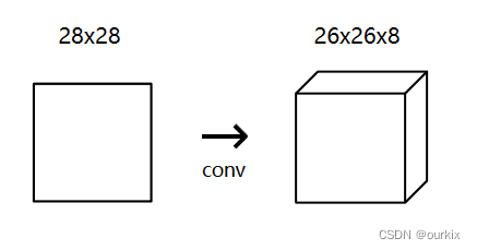
提醒:输出是 26x26x8,而不是 28x28x8,因为我们使用的是有效的填充,这会将输入的宽度和高度减少 2。
conv 层中的 8 个过滤器中的每一个都产生 26x26 的输出,因此它们堆叠在一起构成了一个 26x26x8 的体积。所有这一切的发生都是因为 3×3 (过滤器尺寸)×8(过滤器数量)= 只有 72 个权重!
3.4 实现卷积
是时候将我们学到的知识融入代码了!我们将实现一个 conv 层的前馈部分,该部分负责将过滤器与输入图像进行卷积以生成输出体积。为简单起见,我们假设过滤器始终是 3x3(事实并非如此 - 5x5 和 7x7 过滤器也很常见)。
让我们开始实现一个 conv 层类:
该类只接受一个参数:过滤器的数量。在构造函数中,我们存储过滤器的数量并使用 NumPy 的 randn() 方法初始化一个随机过滤器数组。Conv3x3
注意:在初始化期间,除以 9 比您想象的更重要。如果初始值过大或过小,则训练网络将无效。要了解更多信息,请阅读 Xavier 初始化。
class Conv3x3:
  # A Convolution layer using 3x3 filters.

  def __init__(self, num_filters):
    self.num_filters = num_filters

    # filters is a 3d array with dimensions (num_filters, 3, 3)
    # We divide by 9 to reduce the variance of our initial values
    self.filters = np.random.randn(num_filters, 3, 3) / 9


  def iterate_regions(self, image):
    '''
    Generates all possible 3x3 image regions using valid padding.
    - image is a 2d numpy array
    '''
    h, w = image.shape

    for i in range(h - 2):
      for j in range(w - 2):
        im_region = image[i:(i + 3), j:(j + 3)]
        yield im_region, i, j

  def forward(self, input):
    '''
    Performs a forward pass of the conv layer using the given input.
    Returns a 3d numpy array with dimensions (h, w, num_filters).
    - input is a 2d numpy array
    '''
    input = np.reshape(input, (28, 28))
    self.last_input = input
    h, w = input.shape
    output = np.zeros((h - 2, w - 2, self.num_filters))

    for im_region, i, j in self.iterate_regions(input):
      output[i, j] = np.sum(im_region * self.filters, axis=(1, 2))

    return output


  def backprop(self, d_L_d_out, learn_rate):
    '''
    Performs a backward pass of the conv layer.
    - d_L_d_out is the loss gradient for this layer's outputs.
    - learn_rate is a float.
    '''
    # 初始化一个与滤波器同形状的零数组,用于存储损失函数关于滤波器的梯度。
    d_L_d_filters = np.zeros(self.filters.shape)

    # 这一行是在遍历输入图像的每个区域
    for im_region, i, j in self.iterate_regions(self.last_input):
      # 这一行是在遍历每个滤波器。
      for f in range(self.num_filters):
        #  这一行计算损失函数关于滤波器的梯度。d_L_d_out[i, j, f]
        # 是损失函数关于卷积层输出的梯度,im_region 是输入图像的一个区域。
        # 它们的乘积就是损失函数关于滤波器的梯度,然后累加
        d_L_d_filters[f] += d_L_d_out[i, j, f] * im_region
        #遍历整个图像,将其区域乘以dldout的对应ij元素,并全部累加起来,得出就是一个卷积核大小的东西
    # Update filters
    self.filters -= learn_rate * d_L_d_filters

    # We aren't returning anything here since we use Conv3x3 as
    # the first layer in our CNN. Otherwise, we'd need to return
    # the loss gradient for this layer's inputs, just like every
    # other layer in our CNN.
    return None
iterate_regions()是一种辅助生成器方法,可为我们生成所有有效的 3x3 图像区域。这对于反向传播算法部分很有用。
output[i, j] = np.sum(im_region * self.filters, axis=(1, 2))实际执行卷积的代码。让我们分解一下:
- 我们有一个包含相关图像区域的 3x3 数组。
im_region - 我们有一个 3d 数组。
self.filters - 我们这样做,它使用 numpy 的广播功能将两个数组逐个元素相乘。结果是 与3D 数组的维数相同。
im_region * self.filtersself.filters - np.sum() ,它生成一个长度为 1d 数组,其中每个元素都包含相应滤波器的卷积结果。
axis=(1, 2)num_filters - 我们将结果分配给输出,它包含输出中像素的卷积结果。
output[i, j](i, j)
对输出中的每个像素执行上述,直到我们获得最终的输出体积!让我们对代码进行测试运行:
from mnist import MNIST


#需要将文件解压到固定目录 名称为 t10k-images-idx3-ubyte t10k-lables-idx1-ubyte tran-images-idx3-ubyte  tran-lables-idx1-ubyte ,我是将4个文件文件放到此目录下的C:/Users/Thomas/Desktop/mnistDate
mndata = MNIST('C:/Users/Thomas/Desktop/mnistDate')
train_images, train_labels = mndata.load_training()
test_images, test_labels = mndata.load_testing()


conv = Conv3x3(8)
output = conv.forward(train_images[0])
print(output.shape) # (26, 26, 8)
到目前为止看起来不错。
注意:在我们的实现中,为了简单起见,我们假设输入是一个 2d numpy 数组,因为这就是我们的 MNIST 图像的存储方式。这对我们有用,因为我们将其用作网络中的第一层,但大多数 CNN 都有更多的 Conv 层。如果我们要构建一个需要多次使用的更大网络,我们必须使输入是一个 3d numpy 数组。
Conv3x3
四. 池化
图像中的相邻像素往往具有相似的值,因此卷积图层通常也会为输出中的相邻像素生成相似的值。因此,conv 层输出中包含的大部分信息都是冗余的。例如,如果我们使用边缘检测滤波器并在某个位置找到一条强边缘,那么我们很可能还会在从原始位置偏移 1 个像素的位置找到相对较强的边缘。然而,这些都是相同的优势!我们没有发现任何新东西。
池化层解决了这个问题。他们所做的只是通过(你猜对了)在输入中将值汇集在一起来减少输入的大小。池化通常通过简单的操作(max min average)完成。以下是池化大小为 2 的 Max Pooling 图层的示例:

为了执行最大池化,我们以 2x2 块遍历输入图像(因为池大小 = 2),并将最大值放入输出图像的相应像素处。就是这样!
池化将输入的宽度和高度除以池大小。对于我们的 MNIST CNN,我们将在初始 conv 层之后放置一个池大小为 2 的 Max Pooling 层。池化层会将 26x26x8 的输入转换为 13x13x8 的输出:

4.1 实现池化
我们将使用与上一节中的 conv 类相同的方法实现一个类:MaxPool2
class MaxPool2:
  # A Max Pooling layer using a pool size of 2.

  def iterate_regions(self, image):
    '''
    Generates non-overlapping 2x2 image regions to pool over.
    - image is a 2d numpy array
    '''
    h, w, _ = image.shape
    new_h = h // 2
    new_w = w // 2

    for i in range(new_h):
      for j in range(new_w):
        im_region = image[(i * 2):(i * 2 + 2), (j * 2):(j * 2 + 2)]
        yield im_region, i, j

  def forward(self, input):
    '''
    Performs a forward pass of the maxpool layer using the given input.
    Returns a 3d numpy array with dimensions (h / 2, w / 2, num_filters).
    - input is a 3d numpy array with dimensions (h, w, num_filters)
    '''
    self.last_input = input

    h, w, num_filters = input.shape

    output = np.zeros((h // 2, w // 2, num_filters))

    for im_region, i, j in self.iterate_regions(input):
      output[i, j] = np.amax(im_region, axis=(0, 1))

    return output

  def backprop(self, d_L_d_out):
    '''
    Performs a backward pass of the maxpool layer.
    Returns the loss gradient for this layer's inputs.
    - d_L_d_out is the loss gradient for this layer's outputs.
    '''
    # 将池化前的形状拿出来,全部设置为零
    d_L_d_input = np.zeros(self.last_input.shape)

    # 这一行是在遍历输入图像的每个池化区域
    for im_region, i, j in self.iterate_regions(self.last_input):
      # 获取每个池化区域的高度 h、宽度 w 和过滤器数量 f。
      h, w, f = im_region.shape
      # 计算每个过滤器的最大值。
      amax = np.amax(im_region, axis=(0, 1))

      # 找到最大值保留下来
      for i2 in range(h):
        for j2 in range(w):
          for f2 in range(f):
            # If this pixel was the max value, copy the gradient to it.
            if im_region[i2, j2, f2] == amax[f2]:
              d_L_d_input[i * 2 + i2, j * 2 + j2, f2] = d_L_d_out[i, j, f2]

    return d_L_d_input
这个类的工作方式与我们之前实现的类类似。
关键代码:
output[i, j] = np.amax(im_region, axis=(0, 1))为了从给定的图像区域中找到最大值,我们使用 np.amax(),numpy 的数组 max 方法。我们之所以设置,是因为我们只想在前两个维度(高度和宽度)上最大化,而不是第三个维度。Conv3x3 axis=(0, 1) num_filters
让我们来测试一下吧!
from mnist import MNIST


#需要将文件解压到固定目录 名称为 t10k-images-idx3-ubyte t10k-lables-idx1-ubyte tran-images-idx3-ubyte  tran-lables-idx1-ubyte ,我是将4个文件文件放到此目录下的C:/Users/Thomas/Desktop/mnistDate
mndata = MNIST('C:/Users/Thomas/Desktop/mnistDate')
train_images, train_labels = mndata.load_training()
test_images, test_labels = mndata.load_testing()


conv = Conv3x3(8)
pool = MaxPool2()

output = conv.forward(train_images[0])
output = pool.forward(output)
print(output.shape) # (13, 13, 8)
五. Softmax(软最大化)
为了完成我们的CNN,我们需要赋予它实际进行预测的能力。为此,我们将使用标准的最后一层来解决多类分类问题:Softmax 层,这是一个使用 Softmax 函数作为其激活函数的全连接(密集)层。
提醒:全连接层的每个节点都连接到前一层的每个输出。如果你需要复习一下,我们在神经网络简介中使用了全连接层。
5.1Softmax介绍
如果您以前没有听说过 Softmax,这里详细说下:
Softmax 是将任意实数值转换为概率,这在机器学习中通常很有用。它背后的数学原理非常简单:
给定一些数字,
- 将我们的数字(假设数字为x)变为 e的x次幂。如:数字2,变化后就成了
.
- 将所有指数(的幂)进行相加,作为分母。
- 使用每个数字的幂作为其分子。因为会算出每个值所占概率(这里的概率,数字越大概率越高),所以会轮询计算x1、x2到xn
- 概率 = 分子 除以 分母
公式如下:

s(xi)表示softmax函数,参数xi(是你要算的某个值占据的概率),正常情况会带入x1-xn逐一计算
表示某个值(xi)的e的xi次方
表示将你要计算的所有值的e的(值)次方,全部进行相加求和,
展开了写就是
Softmax 变换的输出始终在[0,1]区间内,并加起来等于 1。因此,它们形成了概率分布。
5.2softmax简单的例子
假设我们有数字 -1、0、3 和 5。
首先,我们计算分母:
分母
然后我们就能计算每个数字所占的概率了:
| x | 分子 ( |
概率 ( |
|---|---|---|
| -1 | 0.002 | |
| 0 | 0.006 | |
| 3 | 0.118 | |
| 5 | 0.874 |
较大的x值会有更高的概率,而且这些所有概率加起来为1.
5.3softmax编程实例
import numpy as np

def softmax(xs):
    return np.exp(xs) / sum(np.exp(xs))

xs = np.array([-1, 0, 3, 5])
print(softmax(xs)) # [0.0021657, 0.00588697, 0.11824302, 0.87370431]
5.4为什么 Softmax 有用?
想象一下,构建一个神经网络来回答这个问题:这张照片是狗还是猫?
这个神经网络的常见设计是让它输出 2 个实数,一个代表狗,另一个代表猫,并对这些值应用 Softmax。例如,假设网络输出[−1,2]
| 动物 | x | 概率 | |
|---|---|---|---|
| 狗 | -1 | 0.368 | 0.047 |
| 猫 | 2 | 7.39 | 0.953 |
这意味着我们的网络有 95.3% 的置信度认为这张照片是一只猫。Softmax 允许我们用概率来回答分类问题,这比更简单的答案(例如二元是/否)更有用。
5.5 用法
我们将使用一个具有 10 个节点的 softmax 层,每个节点代表一个数字,作为 CNN 的最后一层。层中的每个节点都将连接到每个输入。应用softmax变换后,概率最高的节点所表示的数字将是CNN的输出!
5.6 交叉熵损失
您可能会想,为什么要费心将输出转换为概率?输出最大的值不是总是有最大的概率吗?如果你这么认为,你绝对是正确的。我们实际上不需要使用 softmax 来预测数字 - 我们可以从网络中选择输出最大的数字!
softmax真正的作用是帮助我们量化我们对预测的确定性,这在训练和评估我们的CNN时很有用。更具体地说,使用 softmax 可以让我们使用交叉熵损失,它考虑了我们对每个预测的确定性。
什么事交叉熵呢?是香农信息论中一个重要概念,主要用于度量两个概率分布间的差异性信息。
以下是我们计算交叉熵损失的方法:
L是损失函数,前面我们用的是均方误差顺势函数,这里用交叉熵函数。Pc是正确的类的概率(例子中,代表正确的数字的概率),和之前一样这个损失函数输出的值越低越好,例如:
更现实一点,概率可能会是Pc = 0.8,
5.7softmax算法实现
让我们实现softmax层的类
class Softmax:
  # A standard fully-connected layer with softmax activation.

  def __init__(self, input_len, nodes):
    # We divide by input_len to reduce the variance of our initial values
    self.weights = np.random.randn(input_len, nodes) / input_len
    self.biases = np.zeros(nodes)

  def forward(self, input):
    '''
    Performs a forward pass of the softmax layer using the given input.
    Returns a 1d numpy array containing the respective probability values.
    - input can be any array with any dimensions.
    '''
    self.last_input_shape = input.shape

    input = input.flatten()

    self.last_input = input

    input_len, nodes = self.weights.shape

    #这里求出来是一个nodes个数的向量
    totals = np.dot(input, self.weights) + self.biases
    self.last_totals = totals
    #对每个向量进行求e的指数
    exp = np.exp(totals)
    #将求得的值,求和,然后一次求得softmax激活函数的值,形成nodes个向量
    return exp / np.sum(exp, axis=0)

  def backprop(self, d_L_d_out, learn_rate):
    '''
    Performs a backward pass of the softmax layer.
    Returns the loss gradient for this layer's inputs.
    - d_L_d_out is the loss gradient for this layer's outputs.
    '''
    # We know only 1 element of d_L_d_out will be nonzero
    for i, gradient in enumerate(d_L_d_out):
      if gradient == 0:
        continue

      # e^totals
      t_exp = np.exp(self.last_totals)

      # Sum of all e^totals
      S = np.sum(t_exp)

      # Gradients of out[i] against totals
      #选出非零的(也就是类是正确的),求得全为零的倒数,求得正确类的倒数
      d_out_d_t = -t_exp[i] * t_exp / (S ** 2)
      d_out_d_t[i] = t_exp[i] * (S - t_exp[i]) / (S ** 2)

      # Gradients of totals against weights/biases/input
      d_t_d_w = self.last_input
      d_t_d_b = 1
      d_t_d_inputs = self.weights
      # Gradients of loss against totals
      d_L_d_t = gradient * d_out_d_t
      # Gradients of loss against weights/biases/input
      d_L_d_w = d_t_d_w[np.newaxis].T @ d_L_d_t[np.newaxis]
      d_L_d_b = d_L_d_t * d_t_d_b
      d_L_d_inputs = d_t_d_inputs @ d_L_d_t

      # Update weights / biases
      self.weights -= learn_rate * d_L_d_w
      self.biases -= learn_rate * d_L_d_b
      return d_L_d_inputs.reshape(self.last_input_shape)
- input.flatten() 输入扁平化以使其更易于使用,因为我们不再需要它的形状。
- np.dot() 逐个元素相乘,然后对结果求和。
- np.exp() 计算用于 Softmax 的指数。
我们现在已经完成了 CNN 的整个前向传递!把它放在一起:
import mnist
import numpy as np
from conv import Conv3x3
from maxpool import MaxPool2
from softmax import Softmax

# We only use the first 1k testing examples (out of 10k total)
# in the interest of time. Feel free to change this if you want.
test_images = mnist.test_images()[:1000]
test_labels = mnist.test_labels()[:1000]

conv = Conv3x3(8)                  # 28x28x1 -> 26x26x8
pool = MaxPool2()                  # 26x26x8 -> 13x13x8
softmax = Softmax(13 * 13 * 8, 10) # 13x13x8 -> 10

def forward(image, label):
  '''
  Completes a forward pass of the CNN and calculates the accuracy and
  cross-entropy loss.
  - image is a 2d numpy array
  - label is a digit
  '''
  # We transform the image from [0, 255] to [-0.5, 0.5] to make it easier
  # to work with. This is standard practice.
  out = conv.forward((image / 255) - 0.5)
  out = pool.forward(out)
  out = softmax.forward(out)

  # Calculate cross-entropy loss and accuracy. np.log() is the natural log.
  loss = -np.log(out[label])
  acc = 1 if np.argmax(out) == label else 0

  return out, loss, acc

print('MNIST CNN initialized!')

loss = 0
num_correct = 0
for i, (im, label) in enumerate(zip(test_images, test_labels)):
  # Do a forward pass.
  _, l, acc = forward(im, label)
  loss += l
  num_correct += acc

  # Print stats every 100 steps.
  if i % 100 == 99:
    print(
      '[Step %d] Past 100 steps: Average Loss %.3f | Accuracy: %d%%' %
      (i + 1, loss / 100, num_correct)
    )
    loss = 0
    num_correct = 0
运行得出了类似于以下内容:
MNIST CNN initialized!
[Step 100] Past 100 steps: Average Loss 2.302 | Accuracy: 11%
[Step 200] Past 100 steps: Average Loss 2.302 | Accuracy: 8%
[Step 300] Past 100 steps: Average Loss 2.302 | Accuracy: 3%
[Step 400] Past 100 steps: Average Loss 2.302 | Accuracy: 12%
通过随机权重初始化,你会期望CNN只和随机猜测一样好。随机猜测将产生 10% 的准确率(因为有 10 个类)
这就是我们得到的!
六. 训练CNN介绍
训练神经网络通常包括两个阶段:
- 前向传播,输入完全通过网络传递。
- 后向传播,反向传播并更新权重。
我们将遵循此模式来训练我们的 CNN。我们还将使用两个特定的方法:
- 在前向传播,每一层都将缓存后向阶段所需的任何数据(如输入、中间值等)。这意味着任何后向传播之前都必须有相应的正向传播。
- 在后退阶段,每一层将接收一个梯度,并返回一个梯度。它将收到相对于其输出的损失梯度 (
),并返回相对于其输入的损失梯度 (
).
这两个方法将有助于我们的训练整洁有序。了解原因的最好方法可能是查看代码。训练我们的 CNN 最终将如下所示:
# Feed forward
out = conv.forward((image / 255) - 0.5)
out = pool.forward(out)
out = softmax.forward(out)

# Calculate initial gradient
gradient = np.zeros(10)
# ...

# Backprop
gradient = softmax.backprop(gradient)
gradient = pool.backprop(gradient)
gradient = conv.backprop(gradient)
看看它,多漂亮啊,现在想象一下,构建一个有 50 层而不是 3 层的网络——这比拥有良好的系统更有价值。
6.1 反向传播:Softmax
我们将从最后开始,从头开始,因为这就是反向传播的工作方式。首先,回想一下交叉熵损失:
Pc是正确的类别的预测概率。
我们需要计算的是 Softmax 层反向传播的输入,,即损失函数(L)中求得softmax输出(
)的偏导,
是 Softmax 层的输出:10 个概率的向量。下面是损失方程求得的导数(i代表类的遍历,例如,10个类1-10,那么i就从1-10,算出10个结果):
总损失函数求概率p的偏导数,当是正确类的概率时,
=Pc:

代码的实现:
# Calculate initial gradient
gradient = np.zeros(10)
gradient[label] = -1 / out[label]参考前面5.7softmax算法实现中的forward函数,里面有这三句
self.last_input_shape = input.shape

self.last_input = input

self.last_totals = totals
我们在这里缓存了 3 个对实现反向传播有用的东西:
- 存储在将其压平之前的形状数据。
input.shape - 存储压平之后的数据。
input - 总和,即传递给 softmax 激活的值。
这样一来,我们就可以开始推导反向传播阶段的偏导了。我们已经派生了 Softmax 反向传播的输入:.我们可以使用的一个正确的类,因为由上面的公式可知只有正确的类偏导才是非零.这意味着我们除了
可以忽略一切.
这里我们写出的表达式:

当 时,可以写成

这里为了方便理解,画图说明下各个值所代表的意义,假设有两个类,就会有两个神经元节点,输入为三项:


加权求和:
通过激活函数:
解释:是正确类的softmax输出的概率,即上面的P1、P2,
是正确的类的加权求和tc的幂,这里的t1、t2就是我们所说的向量,即在进入激活函数之前的值。
为了加深理解,我们用个例子来说明,计算的表达式,这个即是softmax在正确类时的式子
当softmax()是函数时,假设一共有三个类(x0,x1,x2),x0是正确的类,那么就有softmax(x0),由softmax的公式得出:
我们可以将其他看做常数C,这个式子可以写成:
那么这里求个导数,后面要用到,我们要对x0求导,设softmax(x0)= f(x0):
用除法求导法则得:
用另一种方法来求导数:
我们要求得的是输入到函数的向量,假设这里tc为正确的向量,实际情况中tc为一个常数,我为了区分写成代号,我们设要求的变量为tk,那么我们要求的导数就是上面例子所提到的向量t1、t2的趋势,如下:
那么当神经元节点是处于非正确类的时候,我们求得就是非tc的其他向量的导数,我们的导数公式为:
由于我们已经知道而S又是
这里直接求导数tk有点难,所以用链式法则,所以详细写出来就成了
这里先求,我们带入上面已知的式子得
,这里对S求导,
是常数
所以得
然后求,带入上面的式子得
,这里的
是代表一个变量,是分母求和中的其中一员。为了能够更加清楚的理解,这里展开上面的求和公式得到:
解释下,求和是1-n个类别,所以tk就是这n个里面其中一个,对于tk求导,那么除了tk其他的就其实都是常数。
所以求导得:
那么结合起来求得在输入是非正确类别时的偏导为,
那么当神经元节点是处于正确类的时候,我们求得就是tc的向量的导数,我们的导数公式为:
这里把上面已知式子代入用除法求导公式
展开,
所以这里是直接对式子对变量tc进行求导:
这是整篇文章中最难的一点 - 从这里开始只会变得更容易!
整合上面的两种情况,当输入的类k为正确与非正确是,求得向量t的的偏导公式为:

让我们继续前进。我们最终想要损失与权重、偏差和输入的梯度:
- 我们将使用权重梯度,
,以更新图层的权重。
- 我们将使用偏差梯度,
,以更新我们图层的偏差。
- 我们将返回输入梯度,
,从我们的函数中,以便下一层可以使用它。这是我们在“训练”部分讨论的反向传播!
backprop()
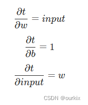
为了计算这 3 个损失梯度,我们首先需要推导出另外 3 个结果:总量与权重、偏差和输入的梯度。这里的相关等式是:
t=W∗input+b
这些渐变很容易!
把所有东西放在一起:

将其放入代码中就不那么简单了,代码部分见 5.7softmax算法实现 中的backprop()函数
     # Gradients of totals against weights/biases/input
      d_t_d_w = self.last_input
      d_t_d_b = 1
      d_t_d_inputs = self.weights
      # Gradients of loss against totals
      d_L_d_t = gradient * d_out_d_t
      # Gradients of loss against weights/biases/input
      d_L_d_w = d_t_d_w[np.newaxis].T @ d_L_d_t[np.newaxis]
      d_L_d_b = d_L_d_t * d_t_d_b
      d_L_d_inputs = d_t_d_inputs @ d_L_d_t
首先,我们预先计算重复使用的变量,因为我们会多次使用它。然后,我们计算每个梯度:
是一维数组。np.newaxis 让我们可以轻松创建一个长度为 1 的新轴,因此我们最终将矩阵与维度 (input_len, 1) 和 (1,nodes ) 相乘。因此
:我们将矩阵与维数 (input_len,nodes ) 和 (nodes, 1) 相乘,得到长度为input_len 的结果。
尝试通过上面计算的小例子,尤其
计算完所有梯度后,剩下的就是实际训练 Softmax 层了!我们将使用随机梯度下降 (SGD) 更新权重和偏差,就像我们在神经网络中所做的那样,然后返回:
请注意,我们添加了一个参数来控制更新权重的速度。此外,我们必须在返回之前这样做,因为我们在前向传递期间扁平化了输入:learn_rate reshape() d_L_d_inputs
      # Update weights / biases
      self.weights -= learn_rate * d_L_d_w
      self.biases -= learn_rate * d_L_d_b
      return d_L_d_inputs.reshape(self.last_input_shape)
6.2Softmax 进行反向传播实例
我们已经完成了第一个 backprop 实现!让我们快速测试一下。我们将开始在文件中实现一个方法:train()
def forward(image, label):
  # Implementation excluded
  # ...

def train(im, label, lr=.005):
  '''
  Completes a full training step on the given image and label.
  Returns the cross-entropy loss and accuracy.
  - image is a 2d numpy array
  - label is a digit
  - lr is the learning rate
  '''
  # Forward
  out, loss, acc = forward(im, label)

  # Calculate initial gradient
  gradient = np.zeros(10)
  gradient[label] = -1 / out[label]

  # Backprop
  gradient = softmax.backprop(gradient, lr)
  # TODO: backprop MaxPool2 layer
  # TODO: backprop Conv3x3 layer

  return loss, acc

print('MNIST CNN initialized!')

# Train!
loss = 0
num_correct = 0
for i, (im, label) in enumerate(zip(train_images, train_labels)):
  if i % 100 == 99:
    print(
      '[Step %d] Past 100 steps: Average Loss %.3f | Accuracy: %d%%' %
      (i + 1, loss / 100, num_correct)
    )
    loss = 0
    num_correct = 0

  l, acc = train(im, label)
  loss += l
  num_correct += acc
运行此命令会得到类似于以下内容的结果:
MNIST CNN initialized!
[Step 100] Past 100 steps: Average Loss 2.239 | Accuracy: 18%
[Step 200] Past 100 steps: Average Loss 2.140 | Accuracy: 32%
[Step 300] Past 100 steps: Average Loss 1.998 | Accuracy: 48%
[Step 400] Past 100 steps: Average Loss 1.861 | Accuracy: 59%
[Step 500] Past 100 steps: Average Loss 1.789 | Accuracy: 56%
[Step 600] Past 100 steps: Average Loss 1.809 | Accuracy: 48%
[Step 700] Past 100 steps: Average Loss 1.718 | Accuracy: 63%
[Step 800] Past 100 steps: Average Loss 1.588 | Accuracy: 69%
[Step 900] Past 100 steps: Average Loss 1.509 | Accuracy: 71%
[Step 1000] Past 100 steps: Average Loss 1.481 | Accuracy: 70%
损失在下降,准确性在上升——我们的 CNN 已经在学习了!
6.3. 反向传播:最大池化 max pooling
Max Pooling 层无法训练,因为它实际上没有任何权重,但我们仍然需要实现一种方法来计算梯度。我们将从再次添加前向传播缓存开始。
这次我们需要缓存的只是输入:详细代码参考 5.7softmax算法实现
class MaxPool2:
  # ...

  def forward(self, input):
    '''
    Performs a forward pass of the maxpool layer using the given input.
    Returns a 3d numpy array with dimensions (h / 2, w / 2, num_filters).
    - input is a 3d numpy array with dimensions (h, w, num_filters)
    '''
    self.last_input = input

    # More implementation
    # ...
在前向传播期间,Max Pooling 图层采用输入体积,并通过选取 2x2 块上的最大值将其宽度和高度尺寸减半。反向传播相反:我们将通过将每个梯度值分配给原始最大值在其相应的 2x2 块中的位置,将损失梯度的宽度和高度加倍。
下面是一个示例。请考虑 Max Pooling 层的以下前向传播:

将 4x4 输入转换为 2x2 输出的前向传播示例
同一层的反向传播如下所示
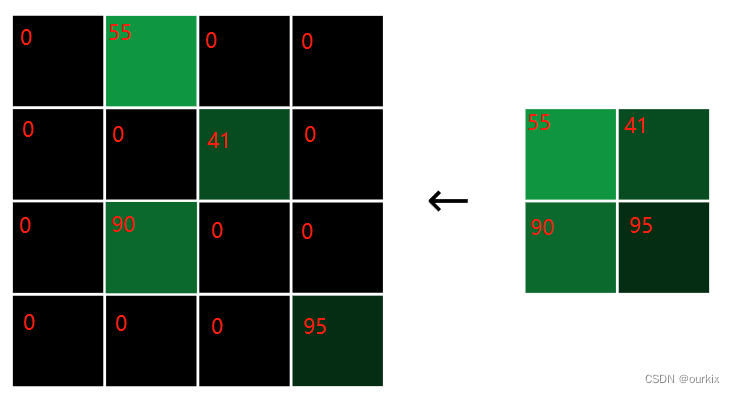
将 2x2 梯度转换为 4x4 梯度的反向传播示例
每个梯度值都分配给原始最大值所在的位置,其他的每个值均为零。上图就是反向传播后的样子
为什么 Max Pooling 层的后退阶段会这样工作?想想为什么,中输入的像素要是不是其 2x2 块中的最大值,对损失的边际影响为零,因为稍微改变该值根本不会改变输出!换言之,
对于非最大像素值来说。另一方面,作为最大值的输入像素会将其值传递到输出,因此
,所以
我们可以使用我们在上面所写的iterate_regions() 方法非常快速地实现。
class MaxPool2:
  # ...

  def iterate_regions(self, image):
    '''
    Generates non-overlapping 2x2 image regions to pool over.
    - image is a 2d numpy array
    '''
    h, w, _ = image.shape
    new_h = h // 2
    new_w = w // 2

    for i in range(new_h):
      for j in range(new_w):
        im_region = image[(i * 2):(i * 2 + 2), (j * 2):(j * 2 + 2)]
        yield im_region, i, j

  def backprop(self, d_L_d_out):
    '''
    Performs a backward pass of the maxpool layer.
    Returns the loss gradient for this layer's inputs.
    - d_L_d_out is the loss gradient for this layer's outputs.
    '''
    d_L_d_input = np.zeros(self.last_input.shape)

    for im_region, i, j in self.iterate_regions(self.last_input):
      h, w, f = im_region.shape
      amax = np.amax(im_region, axis=(0, 1))

      for i2 in range(h):
        for j2 in range(w):
          for f2 in range(f):
            # If this pixel was the max value, copy the gradient to it.
            if im_region[i2, j2, f2] == amax[f2]:
              d_L_d_input[i * 2 + i2, j * 2 + j2, f2] = d_L_d_out[i, j, f2]

    return d_L_d_input
对于每个过滤器中每个 2x2 图像区域中的每个像素,如果它是前向传播期间的最大值,我们将直接把值复制到其原来的对应位置上。
6.4 反向传播:Conv
我们终于来了:通过 Conv 层反向传播是训练 CNN 的核心。
正向传播缓存很简单:
class Conv3x3
  # ...

  def forward(self, input):
    '''
    Performs a forward pass of the conv layer using the given input.
    Returns a 3d numpy array with dimensions (h, w, num_filters).
    - input is a 2d numpy array
    '''
    self.last_input = input

    # More implementation
# ...关于我们实现的提醒:为简单起见,我们假设 conv 层的输入是一个 2d 数组。这只适用于我们,因为我们将其用作网络中的第一层。如果我们要构建一个需要多次使用的更大网络,我们必须使输入为3D数组。
我们主要对 conv 层中过滤器的损失梯度感兴趣,因为我们需要它来更新过滤器权重。我们已经有了对于 conv 层,所以我们只需要计算
.为了计算这一点,我们问自己:改变过滤器的权重将如何影响conv层的输出?
现实情况是,更改任何过滤器权重都会影响经过该过滤器的整个输出图像,因为每个输出像素在卷积过程中都会使用每个像素权重。为了更容易考虑这个问题,让我们一次只考虑一个输出像素:修改过滤器将如何改变一个特定输出像素的输出?
这里有一个超级简单的例子来帮助思考这个问题:
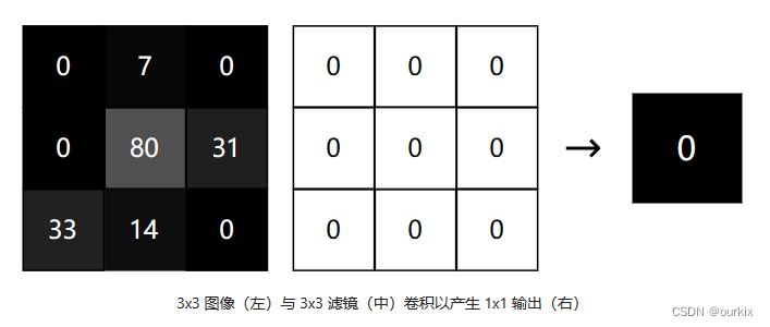
我们有一个 3x3 图像,用一个全零的 3x3 过滤器卷积,以产生 1x1 输出。如果我们将中心过滤器的权重增加 1 会怎样?输出将增加中心图像值 80:

同样,将任何其他过滤器权重增加 1 将使输出增加相应图像像素的值!这表明特定输出像素相对于特定过滤器权重的导数只是相应的图像像素值。下面计算将证实这点

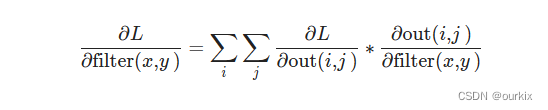
我们将其全部整合在一起,用于计算出特定过滤器的权重梯度
为了加深理解,这里详细说明下如何进行卷积的求导操作的:
假设有一张图片的数据(左)如下,有卷积核(右)如下:
那么卷积的结果就是四个值,具体操作步骤如 三.卷积 中讲述了,
那么假设输入图形的像素值为x1-xn,卷积核的值为w1-wn,
卷积出来的一个像素值表达式可以写成:
所以我们要求过滤器(即卷积核)的某个权重导数就可以表达为:
wi表示w1-wn中某个的值,xi表示为x1-xn中某个的值
由于除了你要求的wi的,其他w都是常数,所以最终求得就是xi的值,即是输入的像素值。
那么对于整个卷积核的导数值就是n次计算所得到的相同卷积核大小的一个矩阵了。其值就是原来的图像,即值为x1-xn。
所以公式写成
那么一张图像进行卷积核求导操作就会进行(图像高-2 * 图像宽度-2)*n这么多次卷积求导运算。我们将这么多次运算排成矩阵,就是整张图的卷积求导输出了
这里将上面的表达式写成更通俗易懂点
,这里的img大小是和卷积核一样大的一个区域,并不是输入的全部原图。
图形的卷积操作可以写成公式: 卷积(img图像,filter卷积核):
这里的out(i,j)指的是卷积后的输出,是一个值,(i,j)为索引表示某个区域的卷积结果
所以可以写成
(i,j)为索引表示某个区域的卷积结果,而内部的求和0-3,是把3x3卷积核的值进行相加(x,y)是进行遍历3x3中的数值。
那么如上所说的,结合起来就能写为:

这样就清晰明了了吧,某个区块的卷积结果的对卷积核求导得到的是这个区块的原输入图像。
那么我们最终要求的其实是损失对卷积核的权重偏导,用链式法则:
这里我们在池化层已经算出来了,所以结果显而易见了
那么我们理一理,的结果是卷积核大小的源输入图像,假设是3x3卷积核。那么结果就是在索引(i,j)位置的3x3大小img。所以要写成
而,由于out在这里是单独一次卷积得出的单一 一个out值,所以写成
,如上面所说out(i,j)是图形卷积后,在out整张图上的(i,j)索引处的一个值。
所以公式写成:
求得的就是卷积核上x,y位置的,对应i,j位置的单个输出的卷积梯度。而由于卷积核会在图像滑动进行计算,所以要求出i,j全部的对应的卷积梯度才是这个卷积核x,y对应的梯度。因为它们都源自L函数中,所以我们要将其相加,这样算出来的就是其真正的卷积梯度了。
然而实际上是一个矩阵,我们上面求得的只是其中一个值,所以实际上
是一个矩阵,
也是一个矩阵。
这里假设out(i,j),i的范围为0-2,j的范围为0-2,那么矩阵就是这样的
同理是这样的,x,y值为要求的卷积核的卷积梯度对应的位置,里面的元素就是由上面公式求得的像素值
那么我们对两个矩阵进行点乘,即两举证对应位置的元素进行相乘,求得矩阵(这里求得就是卷积核滑动过的所有位置的卷积梯度值的一个集合)
因为它们和卷积核的梯度都有关系(是对于像素不同输入的不同结果),我们把他们相加就得到了卷积核的x,y位置的卷积梯度了。。
总结成公式如下:
至此,所有的反向传播都已经讲解完毕了。
(如果有错误请指出,因为包含了个人的学习理解在里面不一定正确)
下面实现conv的反向传播:
class Conv3x3
  # ...

  def backprop(self, d_L_d_out, learn_rate):
    '''
    Performs a backward pass of the conv layer.
    - d_L_d_out is the loss gradient for this layer's outputs.
    - learn_rate is a float.
    '''
    d_L_d_filters = np.zeros(self.filters.shape)

    for im_region, i, j in self.iterate_regions(self.last_input):
      for f in range(self.num_filters):
        d_L_d_filters[f] += d_L_d_out[i, j, f] * im_region

    # Update filters
    self.filters -= learn_rate * d_L_d_filters

    # We aren't returning anything here since we use Conv3x3 as
    # the first layer in our CNN. Otherwise, we'd need to return
    # the loss gradient for this layer's inputs, just like every
    # other layer in our CNN.
    return None
我们通过遍历每个图像区域/过滤器并逐步构建损失梯度来应用我们推导的方程。一旦我们涵盖了所有内容,我们就会像以前一样使用 SGD随机梯度下降 进行更新。
这样,我们就完成了!我们已经通过CNN实现了完整的反向传播。是时候测试一下了......
6. 5训练 CNN
我们将对 CNN 进行几个周期的训练,在训练期间跟踪其进度,然后在单独的测试集上对其进行测试。整个工程的完整代码如下:
import numpy as np
from mnist import MNIST


class Conv3x3:
  # A Convolution layer using 3x3 filters.

  def __init__(self, num_filters):
    self.num_filters = num_filters

    # filters is a 3d array with dimensions (num_filters, 3, 3)
    # We divide by 9 to reduce the variance of our initial values
    self.filters = np.random.randn(num_filters, 3, 3) / 9


  def iterate_regions(self, image):
    '''
    Generates all possible 3x3 image regions using valid padding.
    - image is a 2d numpy array
    '''
    h, w = image.shape

    for i in range(h - 2):
      for j in range(w - 2):
        im_region = image[i:(i + 3), j:(j + 3)]
        yield im_region, i, j

  def forward(self, input):
    '''
    Performs a forward pass of the conv layer using the given input.
    Returns a 3d numpy array with dimensions (h, w, num_filters).
    - input is a 2d numpy array
    '''
    input = np.reshape(input, (28, 28))
    self.last_input = input
    h, w = input.shape
    output = np.zeros((h - 2, w - 2, self.num_filters))

    for im_region, i, j in self.iterate_regions(input):
      output[i, j] = np.sum(im_region * self.filters, axis=(1, 2))

    return output


  def backprop(self, d_L_d_out, learn_rate):
    '''
    Performs a backward pass of the conv layer.
    - d_L_d_out is the loss gradient for this layer's outputs.
    - learn_rate is a float.
    '''
    # 初始化一个与滤波器同形状的零数组,用于存储损失函数关于滤波器的梯度。
    d_L_d_filters = np.zeros(self.filters.shape)

    # 这一行是在遍历输入图像的每个区域
    for im_region, i, j in self.iterate_regions(self.last_input):
      # 这一行是在遍历每个滤波器。
      for f in range(self.num_filters):
        #  这一行计算损失函数关于滤波器的梯度。d_L_d_out[i, j, f]
        # 是损失函数关于卷积层输出的梯度,im_region 是输入图像的一个区域。
        # 它们的乘积就是损失函数关于滤波器的梯度,然后累加
        d_L_d_filters[f] += d_L_d_out[i, j, f] * im_region
        #遍历整个图像,将其区域乘以dldout的对应ij元素,并全部累加起来,得出就是一个卷积核大小的东西
    # Update filters
    self.filters -= learn_rate * d_L_d_filters

    # We aren't returning anything here since we use Conv3x3 as
    # the first layer in our CNN. Otherwise, we'd need to return
    # the loss gradient for this layer's inputs, just like every
    # other layer in our CNN.
    return None


class MaxPool2:
  # A Max Pooling layer using a pool size of 2.

  def iterate_regions(self, image):
    '''
    Generates non-overlapping 2x2 image regions to pool over.
    - image is a 2d numpy array
    '''
    h, w, _ = image.shape
    new_h = h // 2
    new_w = w // 2

    for i in range(new_h):
      for j in range(new_w):
        im_region = image[(i * 2):(i * 2 + 2), (j * 2):(j * 2 + 2)]
        yield im_region, i, j

  def forward(self, input):
    '''
    Performs a forward pass of the maxpool layer using the given input.
    Returns a 3d numpy array with dimensions (h / 2, w / 2, num_filters).
    - input is a 3d numpy array with dimensions (h, w, num_filters)
    '''
    self.last_input = input

    h, w, num_filters = input.shape

    output = np.zeros((h // 2, w // 2, num_filters))

    for im_region, i, j in self.iterate_regions(input):
      output[i, j] = np.amax(im_region, axis=(0, 1))

    return output

  def backprop(self, d_L_d_out):
    '''
    Performs a backward pass of the maxpool layer.
    Returns the loss gradient for this layer's inputs.
    - d_L_d_out is the loss gradient for this layer's outputs.
    '''
    # 将池化前的形状拿出来,全部设置为零
    d_L_d_input = np.zeros(self.last_input.shape)

    # 这一行是在遍历输入图像的每个池化区域
    for im_region, i, j in self.iterate_regions(self.last_input):
      # 获取每个池化区域的高度 h、宽度 w 和过滤器数量 f。
      h, w, f = im_region.shape
      # 计算每个过滤器的最大值。
      amax = np.amax(im_region, axis=(0, 1))

      # 找到最大值保留下来
      for i2 in range(h):
        for j2 in range(w):
          for f2 in range(f):
            # If this pixel was the max value, copy the gradient to it.
            if im_region[i2, j2, f2] == amax[f2]:
              d_L_d_input[i * 2 + i2, j * 2 + j2, f2] = d_L_d_out[i, j, f2]

    return d_L_d_input


class Softmax:
  # A standard fully-connected layer with softmax activation.

  def __init__(self, input_len, nodes):
    # We divide by input_len to reduce the variance of our initial values
    self.weights = np.random.randn(input_len, nodes) / input_len
    self.biases = np.zeros(nodes)

  def forward(self, input):
    '''
    Performs a forward pass of the softmax layer using the given input.
    Returns a 1d numpy array containing the respective probability values.
    - input can be any array with any dimensions.
    '''
    self.last_input_shape = input.shape

    input = input.flatten()

    self.last_input = input

    input_len, nodes = self.weights.shape

    #这里求出来是一个nodes个数的向量
    totals = np.dot(input, self.weights) + self.biases
    self.last_totals = totals
    #对每个向量进行求e的指数
    exp = np.exp(totals)
    #将求得的值,求和,然后一次求得softmax激活函数的值,形成nodes个向量
    return exp / np.sum(exp, axis=0)

  def backprop(self, d_L_d_out, learn_rate):
    '''
    Performs a backward pass of the softmax layer.
    Returns the loss gradient for this layer's inputs.
    - d_L_d_out is the loss gradient for this layer's outputs.
    '''
    # We know only 1 element of d_L_d_out will be nonzero
    for i, gradient in enumerate(d_L_d_out):
      if gradient == 0:
        continue

      # e^totals
      t_exp = np.exp(self.last_totals)

      # Sum of all e^totals
      S = np.sum(t_exp)

      # Gradients of out[i] against totals
      #选出非零的(也就是类是正确的),求得全为零的倒数,求得正确类的倒数
      d_out_d_t = -t_exp[i] * t_exp / (S ** 2)
      d_out_d_t[i] = t_exp[i] * (S - t_exp[i]) / (S ** 2)

      # Gradients of totals against weights/biases/input
      d_t_d_w = self.last_input
      d_t_d_b = 1
      d_t_d_inputs = self.weights
      # Gradients of loss against totals
      d_L_d_t = gradient * d_out_d_t
      # Gradients of loss against weights/biases/input
      d_L_d_w = d_t_d_w[np.newaxis].T @ d_L_d_t[np.newaxis]
      d_L_d_b = d_L_d_t * d_t_d_b
      d_L_d_inputs = d_t_d_inputs @ d_L_d_t

      # Update weights / biases
      self.weights -= learn_rate * d_L_d_w
      self.biases -= learn_rate * d_L_d_b
      return d_L_d_inputs.reshape(self.last_input_shape)


#需要将文件解压到固定目录 名称为 t10k-images-idx3-ubyte t10k-lables-idx1-ubyte tran-images-idx3-ubyte  tran-lables-idx1-ubyte
mndata = MNIST('C:/Users/Thomas/Desktop/mnistDate')
train_images, train_labels = mndata.load_training()
test_images, test_labels = mndata.load_testing()


conv = Conv3x3(8)
pool = MaxPool2()
softmax = Softmax(13 * 13 * 8, 10) # 13x13x8 -> 10


def forward(image, label):
  '''
  Completes a forward pass of the CNN and calculates the accuracy and
  cross-entropy loss.
  - image is a 2d numpy array
  - label is a digit
  '''
  # We transform the image from [0, 255] to [-0.5, 0.5] to make it easier
  # to work with. This is standard practice.
  image =  np.reshape(image, (28, 28))
  out = conv.forward((image / 255) - 0.5)
  out = pool.forward(out)
  out = softmax.forward(out)

  # Calculate cross-entropy loss and accuracy. np.log() is the natural log.
  loss = -np.log(out[label])
  acc = 1 if np.argmax(out) == label else 0

  return out, loss, acc


def train(im, label, lr=.005):
  '''
  Completes a full training step on the given image and label.
  Returns the cross-entropy loss and accuracy.
  - image is a 2d numpy array
  - label is a digit
  - lr is the learning rate
  '''
  # Forward
  out, loss, acc = forward(im, label)

  # Calculate initial gradient
  gradient = np.zeros(10)
  gradient[label] = -1 / out[label]

 # Backprop
  gradient = softmax.backprop(gradient, lr)
  gradient = pool.backprop(gradient)
  gradient = conv.backprop(gradient, lr)

  return loss, acc

print('MNIST CNN initialized!')

# Train the CNN for 3 epochs
for epoch in range(3):
  print('--- Epoch %d ---' % (epoch + 1))

  # Shuffle the training data
  permutation = np.random.permutation(len(train_images))
  train_images1 = train_images[permutation]
  train_labels1 = train_labels[permutation]

  # Train!
  loss = 0
  num_correct = 0
  for i, (im, label) in enumerate(zip(train_images1, train_labels1)):
    if i > 0 and i % 100 == 99:
      print(
        '[Step %d] Past 100 steps: Average Loss %.3f | Accuracy: %d%%' %
        (i + 1, loss / 100, num_correct)
      )
      loss = 0
      num_correct = 0

    l, acc = train(im, label)
    loss += l
    num_correct += acc

# Test the CNN
print('\n--- Testing the CNN ---')
loss = 0
num_correct = 0
for im, label in zip(test_images, test_labels):
  _, l, acc = forward(im, label)
  loss += l
  num_correct += acc

num_tests = len(test_images)
print('Test Loss:', loss / num_tests)
print('Test Accuracy:', num_correct / num_tests)
运行代码的输出示例:
MNIST CNN initialized!
--- Epoch 1 ---
[Step 100] Past 100 steps: Average Loss 2.254 | Accuracy: 18%
[Step 200] Past 100 steps: Average Loss 2.167 | Accuracy: 30%
[Step 300] Past 100 steps: Average Loss 1.676 | Accuracy: 52%
[Step 400] Past 100 steps: Average Loss 1.212 | Accuracy: 63%
[Step 500] Past 100 steps: Average Loss 0.949 | Accuracy: 72%
[Step 600] Past 100 steps: Average Loss 0.848 | Accuracy: 74%
[Step 700] Past 100 steps: Average Loss 0.954 | Accuracy: 68%
[Step 800] Past 100 steps: Average Loss 0.671 | Accuracy: 81%
[Step 900] Past 100 steps: Average Loss 0.923 | Accuracy: 67%
[Step 1000] Past 100 steps: Average Loss 0.571 | Accuracy: 83%
--- Epoch 2 ---
[Step 100] Past 100 steps: Average Loss 0.447 | Accuracy: 89%
[Step 200] Past 100 steps: Average Loss 0.401 | Accuracy: 86%
[Step 300] Past 100 steps: Average Loss 0.608 | Accuracy: 81%
[Step 400] Past 100 steps: Average Loss 0.511 | Accuracy: 83%
[Step 500] Past 100 steps: Average Loss 0.584 | Accuracy: 89%
[Step 600] Past 100 steps: Average Loss 0.782 | Accuracy: 72%
[Step 700] Past 100 steps: Average Loss 0.397 | Accuracy: 84%
[Step 800] Past 100 steps: Average Loss 0.560 | Accuracy: 80%
[Step 900] Past 100 steps: Average Loss 0.356 | Accuracy: 92%
[Step 1000] Past 100 steps: Average Loss 0.576 | Accuracy: 85%
--- Epoch 3 ---
[Step 100] Past 100 steps: Average Loss 0.367 | Accuracy: 89%
[Step 200] Past 100 steps: Average Loss 0.370 | Accuracy: 89%
[Step 300] Past 100 steps: Average Loss 0.464 | Accuracy: 84%
[Step 400] Past 100 steps: Average Loss 0.254 | Accuracy: 95%
[Step 500] Past 100 steps: Average Loss 0.366 | Accuracy: 89%
[Step 600] Past 100 steps: Average Loss 0.493 | Accuracy: 89%
[Step 700] Past 100 steps: Average Loss 0.390 | Accuracy: 91%
[Step 800] Past 100 steps: Average Loss 0.459 | Accuracy: 87%
[Step 900] Past 100 steps: Average Loss 0.316 | Accuracy: 92%
[Step 1000] Past 100 steps: Average Loss 0.460 | Accuracy: 87%

--- Testing the CNN ---
Test Loss: 0.5979384893783474
Test Accuracy: 0.78
我们的代码有效!在短短 3000 个训练步骤中,我们从损失 2.3 和 10% 准确率的模型增加到 0.6 损失和 78% 的准确率。