import numpy as np
import pandas as pd
import torch as t
from PIL import Image
from torchvision.transforms import ToTensor, ToPILImage

t.__version__
'2.1.1'
3.1 图像相关层
图像相关层主要包括卷积层(Conv)、池化层(Pool)等,这些层在实际使用中可分为一维(1D)、二维(2D)、三维(3D),池化方式又分为平均池化(AvgPool)、最大值池化(MaxPool)、自适应池化(AdaptiveAvgPool)等。而卷积层除了常用的前向卷积之外,还有逆卷积(TransposeConv)。
除了这里的使用,图像的卷积操作还有各种变体,具体可以参照此处动图[^2]介绍。 [^2]: https://github.com/vdumoulin/conv_arithmetic/blob/master/README.md
to_tensor = ToTensor()
to_pil = ToPILImage()
lena = Image.open('imgs/lena.png')
lena

# layer对输入形状都有假设:输入的不是单个数据,而是一个batch。
# 这里输入一个数据,就必须调用tensor.unsqueeze(0)增加一个维度,伪装成batch_size=1的batch
input = to_tensor(lena).unsqueeze(0)

# 锐化卷积核
kernel = t.ones(3, 3) / -9
kernel[1][1] = 1
conv = t.nn.Conv2d(1, 1, (3, 3), 1, bias=False)
conv.weight.data = kernel.view(1, 1, 3, 3)

out = conv(input)
to_pil(out.data.squeeze(0))

池化层:可视为一种特殊的卷积层,用来下采样。注意池化层是没有可学习参数的,其weight是固定的。
pool = t.nn.AvgPool2d(2, 2)
out = pool(input)
to_pil(out.data.squeeze(0))

除了卷积层和池化层,深度学习中还将常用到以下几个层:
- Linear:全连接层。
- BatchNorm:批规范化层,分为1D、2D和3D。除了标准的BatchNorm之外,还有在风格迁移中常用到的InstanceNorm层。
- Dropout:dropout层,用来防止过拟合,同样分为1D、2D和3D。
下面通过例子来说明它们的使用。
# 输入batch_size=2, 维度3
input = t.rand(2,3)
linear = t.nn.Linear(3, 4)
h = linear(input)
h
tensor([[-0.2314, -0.2245,  0.0966,  0.7610],
        [-0.2679, -0.2403,  0.0086,  0.5799]], grad_fn=<AddmmBackward0>)
# 4 channel,初始化标准差4,均值0
bn = t.nn.BatchNorm1d(4)
bn.weight.data = t.ones(4) * 4
bn.bias.data = t.zeros(4)

bn_out = bn(h)
print(bn_out)
bn_out.mean(), bn_out.var(0, unbiased=False)       # 由于计算无偏方差分母会减1, 使用unbiased=1分母不减一
tensor([[ 3.9415,  3.7136,  3.9897,  3.9976],
        [-3.9415, -3.7136, -3.9897, -3.9976]],
       grad_fn=<NativeBatchNormBackward0>)


(tensor(-1.8775e-06, grad_fn=<MeanBackward0>),
 tensor([15.5355, 13.7908, 15.9179, 15.9805], grad_fn=<VarBackward0>))
# 每个元素以0.5的概率舍弃
dropout = t.nn.Dropout(0.5)
o = dropout(bn_out)
o
tensor([[ 7.8830,  7.4272,  0.0000,  7.9951],
        [-7.8830, -7.4272, -7.9794, -7.9951]], grad_fn=<MulBackward0>)
3.2 激活函数
PyTorch实现了常见的激活函数,其具体的接口信息可参见官方文档1,这些激活函数可作为独立的layer使用。这里将介绍最常用的激活函数ReLU,其数学表达式为:
R e L U ( x ) = m a x ( 0 , x ) ReLU(x)=max(0,x) ReLU(x)=max(0,x)
ReLU函数有个inplace参数,如果设为True,它会把输出直接覆盖到输入中,这样可以节省内存/显存。之所以可以覆盖是因为在计算ReLU的反向传播时,只需根据输出就能够推算出反向传播的梯度。但是只有少数的autograd操作支持inplace操作(如tensor.sigmoid_()),除非你明确地知道自己在做什么,否则一般不要使用inplace操作。
relu = t.nn.ReLU(inplace=True)
input = t.randn(2, 3)
print(input)
output = relu(input)
print(output)        # 负数都被截断为0
tensor([[-0.4064, -0.1886,  0.4812],
        [ 0.8996, -0.3606,  0.6127]])
tensor([[0.0000, 0.0000, 0.4812],
        [0.8996, 0.0000, 0.6127]])
对于此类网络如果每次都写复杂的forward函数会有些麻烦,在此就有两种简化方式,ModuleList和Sequential。其中Sequential是一个特殊的module,它包含几个子Module,前向传播时会将输入一层接一层的传递下去。ModuleList也是一个特殊的module,可以包含几个子module,可以像用list一样使用它,但不能直接把输入传给ModuleList。下面举例说明。
# Sequential
net = t.nn.Sequential(
    t.nn.Conv2d(3, 3, 3),
    t.nn.BatchNorm2d(3),
    t.nn.ReLU()
)
print('net:', net)
net: Sequential(
  (0): Conv2d(3, 3, kernel_size=(3, 3), stride=(1, 1))
  (1): BatchNorm2d(3, eps=1e-05, momentum=0.1, affine=True, track_running_stats=True)
  (2): ReLU()
)
# 可根据名字或序号取出module
net[2]
ReLU()
input = t.randn(1, 3, 4, 4)
output = net(input)
output
tensor([[[[1.2239, 0.0000],
          [0.0000, 0.6354]],

         [[0.1855, 0.0000],
          [0.7218, 0.7777]],

         [[1.3686, 0.0000],
          [0.4861, 0.0000]]]], grad_fn=<ReluBackward0>)
# modellist
modellist = t.nn.ModuleList([t.nn.Linear(3, 4), t.nn.ReLU(), t.nn.Linear(4, 2)])
input = t.randn(1, 3)

for model in modellist:
    input = model(input)
    print(input)
tensor([[-0.1817,  0.3852,  1.3656, -0.5643]], grad_fn=<AddmmBackward0>)
tensor([[0.0000, 0.3852, 1.3656, 0.0000]], grad_fn=<ReluBackward0>)
tensor([[-0.0151, -0.0309]], grad_fn=<AddmmBackward0>)
3.3 RNN循环神经网络
关于RNN的基础知识,推荐阅读colah的文章2入门。PyTorch中实现了如今最常用的三种RNN:RNN(vanilla RNN)、LSTM和GRU。此外还有对应的三种RNNCell。
RNN和RNNCell层的区别在于前者一次能够处理整个序列,而后者一次只处理序列中一个时间点的数据,前者封装更完备更易于使用,后者更具灵活性。实际上RNN层的一种后端实现方式就是调用RNNCell来实现的。
t.manual_seed(1000)
# 输入:batch_size=3, 序列长度为2,序列中每个元素占4维
input = t.randn(2, 3, 4)
# lstm输入向量4维,隐藏元3. 1层
lstm = t.nn.LSTM(4, 3, 1)
# 初始状态:1层,batch_size=3, 3个隐藏元
h0 = t.randn(1, 3, 3)
c0 = t.randn(1, 3, 3)
out, hn = lstm(input, (h0, c0))
out
tensor([[[-0.3610, -0.1643,  0.1631],
         [-0.0613, -0.4937, -0.1642],
         [ 0.5080, -0.4175,  0.2502]],

        [[-0.0703, -0.0393, -0.0429],
         [ 0.2085, -0.3005, -0.2686],
         [ 0.1482, -0.4728,  0.1425]]], grad_fn=<MkldnnRnnLayerBackward0>)
t.manual_seed(1000)
input = t.randn(2, 3, 4)
# 一个LSTMCell对应的层数只能是一层
lstm = t.nn.LSTMCell(4, 3)
hx = t.randn(3, 3)
cx = t.randn(3, 3)
out = []
for i_ in input:
    hx, cx=lstm(i_, (hx, cx))
    out.append(hx)
t.stack(out)
tensor([[[-0.3610, -0.1643,  0.1631],
         [-0.0613, -0.4937, -0.1642],
         [ 0.5080, -0.4175,  0.2502]],

        [[-0.0703, -0.0393, -0.0429],
         [ 0.2085, -0.3005, -0.2686],
         [ 0.1482, -0.4728,  0.1425]]], grad_fn=<StackBackward0>)
3.4 损失函数
损失函数可看作是一种特殊的layer,PyTorch也将这些损失函数实现为nn.Module的子类。然而在实际使用中通常将这些loss function专门提取出来,和主模型互相独立。详细的loss使用请参照文档3,这里以分类中最常用的交叉熵损失CrossEntropyloss为例说明。
# batch_size = 3, 计算对应每个类别的分数(只有两个类别)
score = t.randn(3, 2)
# 三个样本分别属于1, 0, 1类,label必须是LongTensor
label = t.Tensor([1, 0, 1]).long()

# loss与普通的layer无差异
criterion = t.nn.CrossEntropyLoss()
loss = criterion(score, label)
loss
tensor(1.8772)