SHAP（五）：使用 XGBoost 进行人口普查收入分类

2023-12-06 22:50:03
开发
37

SHAP（五）：使用 XGBoost 进行人口普查收入分类

本笔记本演示了如何使用 XGBoost 预测个人年收入超过 5 万美元的概率。它使用标准 UCI 成人收入数据集。要下载此笔记本的副本，请访问 github。

XGBoost 等梯度增强机方法对于具有多种形式的表格样式输入数据的此类预测问题来说是最先进的。 Tree SHAP（arXiv 论文）允许精确计算树集成方法的 SHAP 值，并已直接集成到 C++ XGBoost 代码库中。这允许快速精确计算 SHAP 值，无需采样，也无需提供背景数据集（因为背景是从树木的覆盖范围推断出来的）。

在这里，我们演示如何使用 SHAP 值来理解 XGBoost 模型预测。

import matplotlib.pylab as pl
import numpy as np
import xgboost
from sklearn.model_selection import train_test_split

import shap

# print the JS visualization code to the notebook
shap.initjs()

1.加载数据集

X, y = shap.datasets.adult()
X_display, y_display = shap.datasets.adult(display=True)

# create a train/test split
X_train, X_test, y_train, y_test = train_test_split(X, y, test_size=0.2, random_state=7)
d_train = xgboost.DMatrix(X_train, label=y_train)
d_test = xgboost.DMatrix(X_test, label=y_test)

2.训练模型

params = {
   
    "eta": 0.01,
    "objective": "binary:logistic",
    "subsample": 0.5,
    "base_score": np.mean(y_train),
    "eval_metric": "logloss",
}
model = xgboost.train(
    params,
    d_train,
    5000,
    evals=[(d_test, "test")],
    verbose_eval=100,
    early_stopping_rounds=20,
)

[0]	test-logloss:0.54663
[100]	test-logloss:0.36373
[200]	test-logloss:0.31793
[300]	test-logloss:0.30061
[400]	test-logloss:0.29207
[500]	test-logloss:0.28678
[600]	test-logloss:0.28381
[700]	test-logloss:0.28181
[800]	test-logloss:0.28064
[900]	test-logloss:0.27992
[1000]	test-logloss:0.27928
[1019]	test-logloss:0.27935

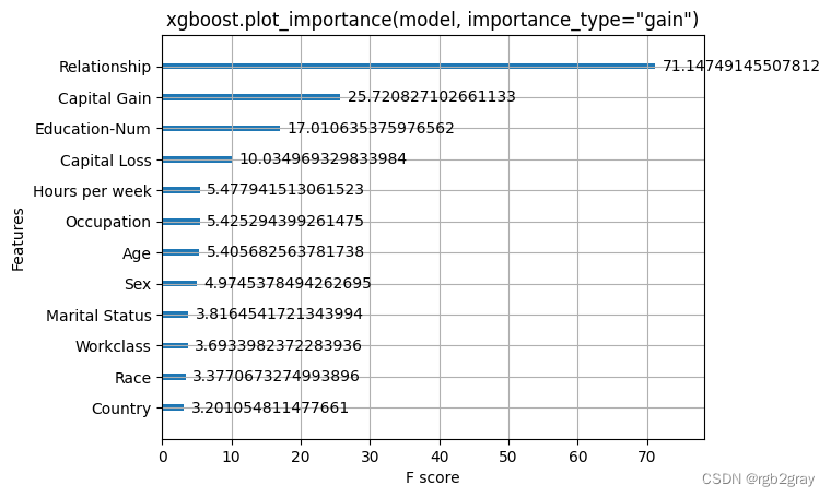
3.经典特征归因

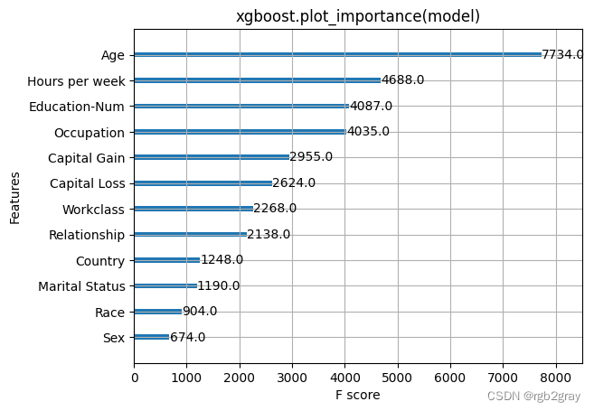
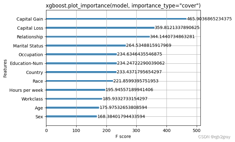
在这里，我们尝试 XGBoost 附带的全局特征重要性计算。请注意，它们都是相互矛盾的，这激励了 SHAP 值的使用，因为它们具有一致性保证（意味着它们将正确排序特征）。

xgboost.plot_importance(model)
pl.title("xgboost.plot_importance(model)")
pl.show()

在这里插入图片描述

xgboost.plot_importance(model, importance_type="cover")
pl.title('xgboost.plot_importance(model, importance_type="cover")')
pl.show()

在这里插入图片描述

xgboost.plot_importance(model, importance_type="gain")
pl.title('xgboost.plot_importance(model, importance_type="gain")')
pl.show()

在这里插入图片描述

4,解释预测

在这里，我们使用集成到 XGBoost 中的 Tree SHAP 实现来解释整个数据集（32561 个样本）。

# this takes a minute or two since we are explaining over 30 thousand samples in a model with over a thousand trees
explainer = shap.TreeExplainer(model)
shap_values = explainer.shap_values(X)

4.1 可视化单个预测

请注意，我们使用“显示值”数据框，因此我们得到了漂亮的字符串而不是类别代码。

shap.force_plot(explainer.expected_value, shap_values[0, :], X_display.iloc[0, :])

在这里插入图片描述

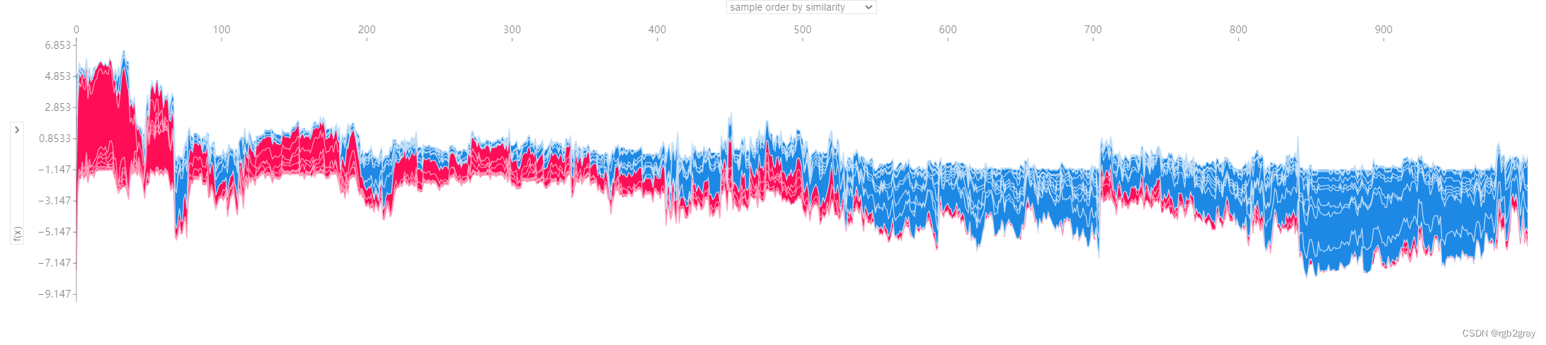
4.2 将许多预测可视化

为了让浏览器满意，我们只可视化 1,000 个人。

shap.force_plot(
    explainer.expected_value, shap_values[:1000, :], X_display.iloc[:1000, :]
)

在这里插入图片描述

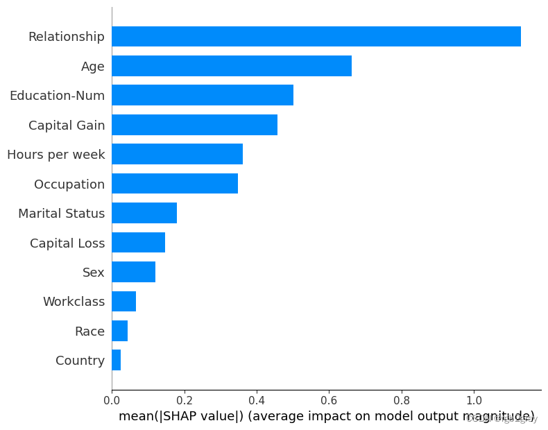
5.平均重要性条形图

这取整个数据集中 SHAP 值大小的平均值，并将其绘制为简单的条形图。

shap.summary_plot(shap_values, X_display, plot_type="bar")

在这里插入图片描述

6.SHAP 概要图

我们没有使用典型的特征重要性条形图，而是使用每个特征的 SHAP 值的密度散点图来确定每个特征对验证数据集中个体的模型输出有多大影响。特征按所有样本的 SHAP 值大小之和排序。有趣的是，关系特征比资本收益特征具有更大的总体模型影响，但对于那些资本收益重要的样本，它比年龄具有更大的影响。换句话说，资本收益对少数预测的影响较大，而年龄对所有预测的影响较小。

请注意，当散点不适合在线时，它们会堆积起来以显示密度，每个点的颜色代表该个体的特征值。

shap.summary_plot(shap_values, X)

在这里插入图片描述

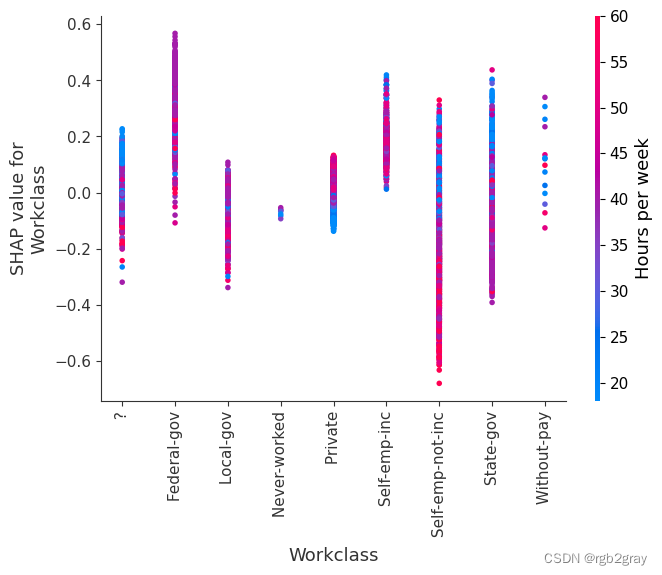
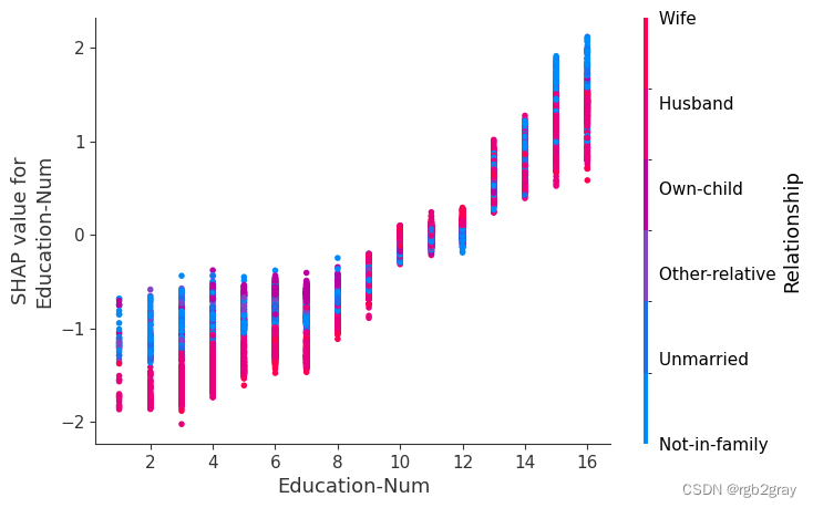
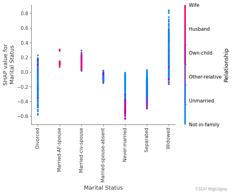
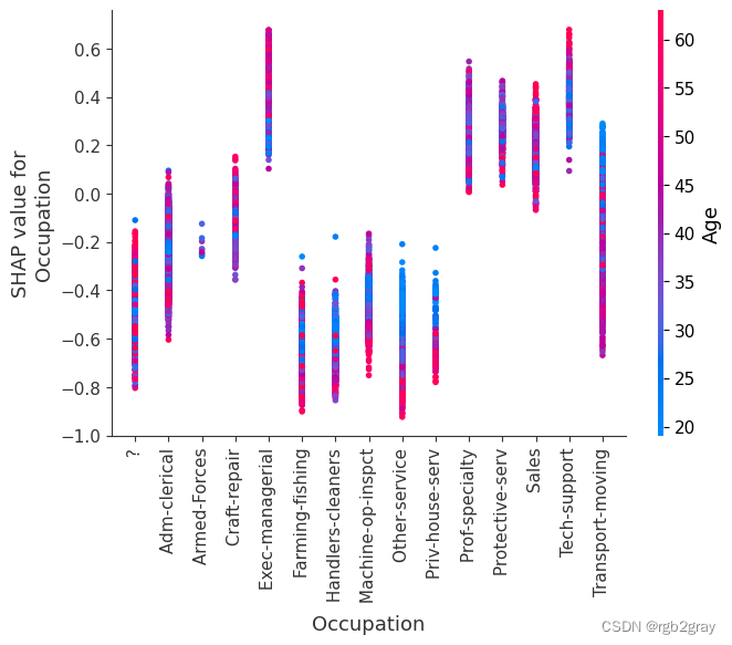
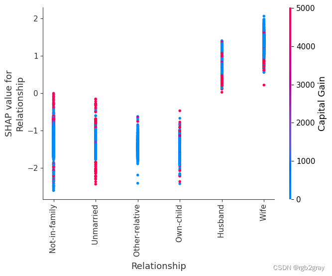
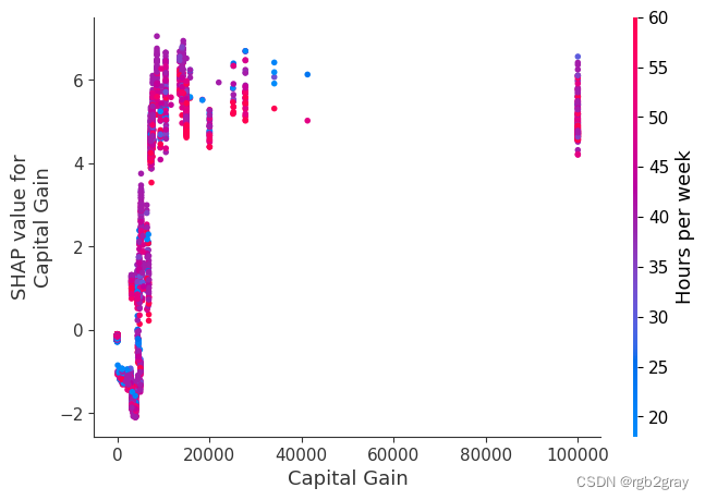
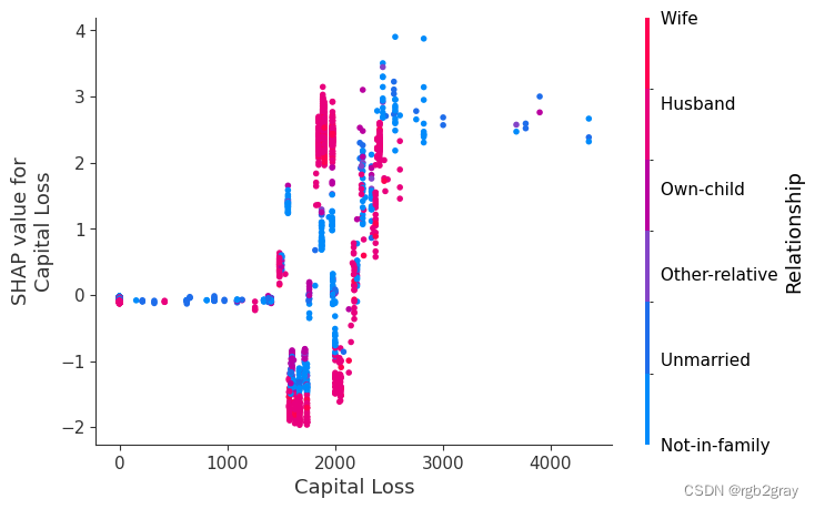
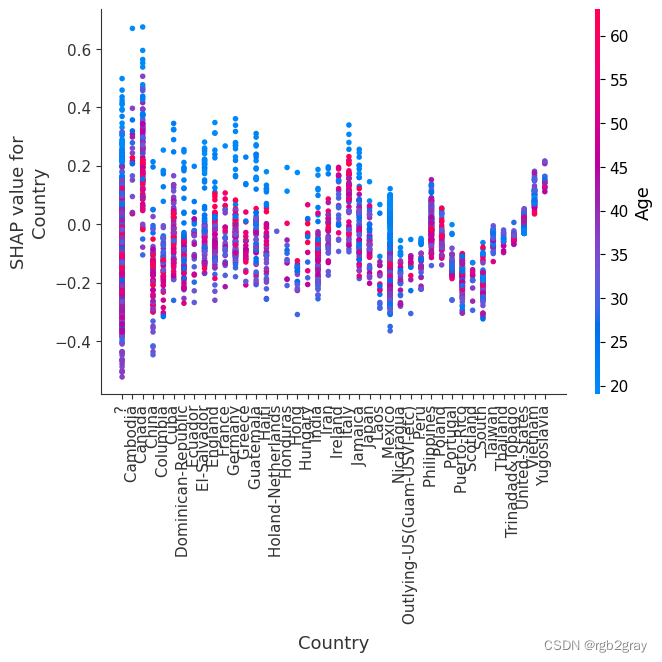
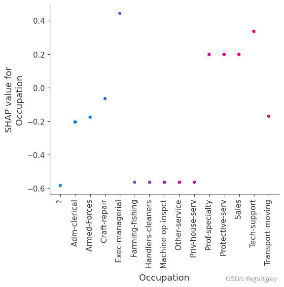
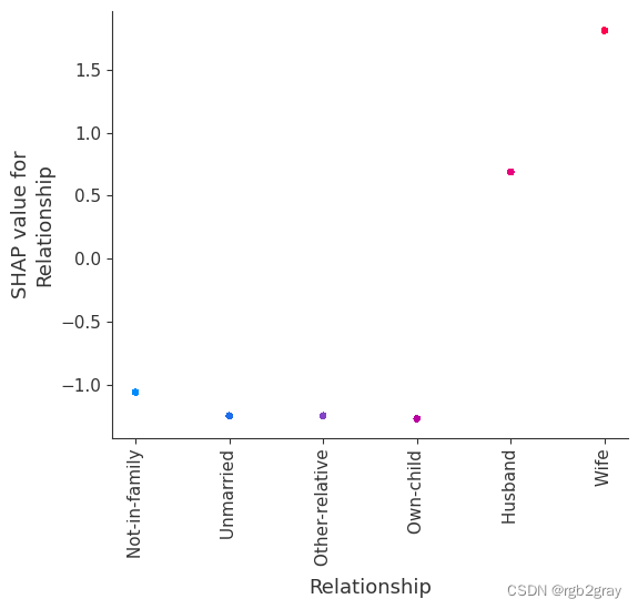
7.SHAP 相关图

SHAP 依赖图显示单个特征对整个数据集的影响。他们绘制了多个样本中某个特征的值与该特征的 SHA 值的关系图。 SHAP 依赖图与部分依赖图类似，但考虑了特征中存在的交互效应，并且仅在数据支持的输入空间区域中定义。单个特征值处的 SHAP 值的垂直分散是由交互效应驱动的，并且选择另一个特征进行着色以突出可能的交互。

for name in X_train.columns:
    shap.dependence_plot(name, shap_values, X, display_features=X_display)

在这里插入图片描述

在这里插入图片描述
)

在这里插入图片描述

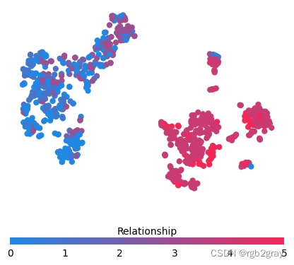
8.简单的监督聚类

按 shap_values 对人们进行聚类会导致与手头的预测任务相关的组（在本例中是他们的收入潜力）。

from sklearn.decomposition import PCA
from sklearn.manifold import TSNE

shap_pca50 = PCA(n_components=12).fit_transform(shap_values[:1000, :])
shap_embedded = TSNE(n_components=2, perplexity=50).fit_transform(shap_values[:1000, :])

from matplotlib.colors import LinearSegmentedColormap

cdict1 = {
   
    "red": (
        (0.0, 0.11764705882352941, 0.11764705882352941),
        (1.0, 0.9607843137254902, 0.9607843137254902),
    ),
    "green": (
        (0.0, 0.5333333333333333, 0.5333333333333333),
        (1.0, 0.15294117647058825, 0.15294117647058825),
    ),
    "blue": (
        (0.0, 0.8980392156862745, 0.8980392156862745),
        (1.0, 0.3411764705882353, 0.3411764705882353),
    ),
    "alpha": ((0.0, 1, 1), (0.5, 1, 1), (1.0, 1, 1)),
}  # #1E88E5 -> #ff0052
red_blue_solid = LinearSegmentedColormap("RedBlue", cdict1)

f = pl.figure(figsize=(5, 5))
pl.scatter(
    shap_embedded[:, 0],
    shap_embedded[:, 1],
    c=shap_values[:1000, :].sum(1).astype(np.float64),
    linewidth=0,
    alpha=1.0,
    cmap=red_blue_solid,
)
cb = pl.colorbar(label="Log odds of making > $50K", aspect=40, orientation="horizontal")
cb.set_alpha(1)
cb.outline.set_linewidth(0)
cb.ax.tick_params("x", length=0)
cb.ax.xaxis.set_label_position("top")
pl.gca().axis("off")
pl.show()

在这里插入图片描述

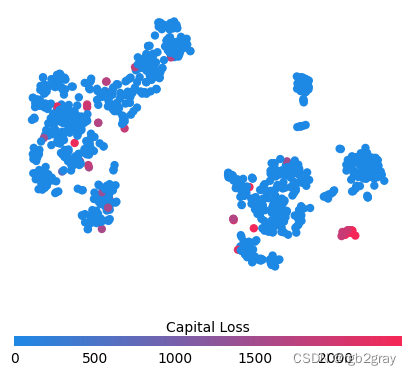
for feature in ["Relationship", "Capital Gain", "Capital Loss"]:
    f = pl.figure(figsize=(5, 5))
    pl.scatter(
        shap_embedded[:, 0],
        shap_embedded[:, 1],
        c=X[feature].values[:1000].astype(np.float64),
        linewidth=0,
        alpha=1.0,
        cmap=red_blue_solid,
    )
    cb = pl.colorbar(label=feature, aspect=40, orientation="horizontal")
    cb.set_alpha(1)
    cb.outline.set_linewidth(0)
    cb.ax.tick_params("x", length=0)
    cb.ax.xaxis.set_label_position("top")
    pl.gca().axis("off")
    pl.show()

在这里插入图片描述

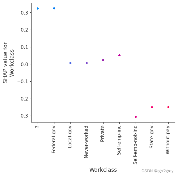
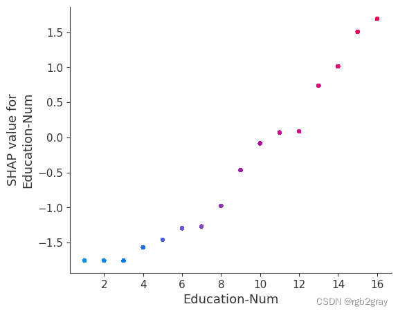
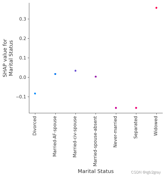
训练每棵树只有两个叶子的模型，因此特征之间没有交互项

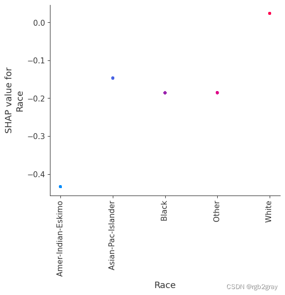
强制模型没有交互项意味着某个特征对结果的影响不依赖于任何其他特征的值。这反映在下面的 SHAP 相关图中，因为没有垂直扩展。垂直分布反映了一个特征的单个值可能对模型输出产生不同的影响，具体取决于个体呈现的其他特征的上下文。然而，对于没有交互项的模型，无论个体可能具有哪些其他属性，特征总是具有相同的影响。

与传统的部分相关图相比，SHAP 相关图的优点之一是能够区分具有交互项和不具有交互项的模型。换句话说，SHAP 相关图通过给定特征值处散点图的垂直方差给出了交互项大小的概念。

# train final model on the full data set
params = {
   
    "eta": 0.05,
    "max_depth": 1,
    "objective": "binary:logistic",
    "subsample": 0.5,
    "base_score": np.mean(y_train),
    "eval_metric": "logloss",
}
model_ind = xgboost.train(
    params,
    d_train,
    5000,
    evals=[(d_test, "test")],
    verbose_eval=100,
    early_stopping_rounds=20,
)

[0]	test-logloss:0.54113
[100]	test-logloss:0.35499
[200]	test-logloss:0.32848
[300]	test-logloss:0.31901
[400]	test-logloss:0.31331
[500]	test-logloss:0.30930
[600]	test-logloss:0.30619
[700]	test-logloss:0.30371
[800]	test-logloss:0.30184
[900]	test-logloss:0.30035
[1000]	test-logloss:0.29913
[1100]	test-logloss:0.29796
[1200]	test-logloss:0.29695
[1300]	test-logloss:0.29606
[1400]	test-logloss:0.29525
[1500]	test-logloss:0.29471
[1565]	test-logloss:0.29439

shap_values_ind = shap.TreeExplainer(model_ind).shap_values(X)

请注意，下面的交互颜色条对于该模型来说没有意义，因为它没有交互。

for name in X_train.columns:
    shap.dependence_plot(name, shap_values_ind, X, display_features=X_display)

invalid value encountered in divide
invalid value encountered in divide

在这里插入图片描述

invalid value encountered in divide
invalid value encountered in divide

在这里插入图片描述

invalid value encountered in divide
invalid value encountered in divide

在这里插入图片描述

invalid value encountered in divide
invalid value encountered in divide

在这里插入图片描述

invalid value encountered in divide
invalid value encountered in divide

在这里插入图片描述

invalid value encountered in divide
invalid value encountered in divide

在这里插入图片描述

invalid value encountered in divide
invalid value encountered in divide

在这里插入图片描述

原文地址:https://blog.csdn.net/weixin_44026026/article/details/134758214 本文来自互联网用户投稿，该文观点仅代表作者本人，不代表本站立场。本站仅提供信息存储空间服务，不拥有所有权，不承担相关法律责任。如若转载，请注明出处：https://www.suanlizi.com/kf/1732412088367845376.html 如若内容造成侵权/违法违规/事实不符，请联系《酸梨子》网邮箱：1419361763@qq.com进行投诉反馈，一经查实，立即删除！

阅读全部