文章目录
将三维空间中的点云使用 BEV 的方式多视角投影到某个平面之后,可能需要用到该平面投影图(光栅化之前)的点集的凸包,所以这里记录一下常见的 graham 凸包算法。
向量的内积(点乘)、外积(叉乘)
graham 算法模拟最外层点集包围的过程的关键思想是使用两个向量之间的外积来判断下一条连线的转角,如果向外拐了,那说明当前基点在本次连线之后会成为一块凹陷,注意“凸包”的定义,每个顶角的角度都小于 18 0 ∘ 180^\circ 180∘ 才叫 “凸” ,如果有一个内凹顶点,那么它的内角是大于 18 0 ∘ 180^\circ 180∘ 的,可以确定,它应该是包含在实际的最终计算出来的理想凸包之内才对,这个时候就需要调整连线的基点为上一个基点。
在二维平面上,叉积的结果与向量的顺时针或逆时针旋转方向有关。具体来说:
- 对于二维平面上的两个向量 u = ( x 1 , y 1 ) u=(x_1,y_1) u=(x1,y1) 和 v = ( x 2 , y 2 ) v=(x_2, y_2) v=(x2,y2) ,它们的叉积可以使用一个标量值来表示 u × v = x 1 y 2 − y 1 x 2 u\times v = x_1y_2 - y_1x_2 u×v=x1y2−y1x2
- 这个标量值表示了这两个向量所定义的平行四边形的有向面积,也可以用来判定向量的旋转方向。
确定旋转方向
- 正值:当 叉积 的值为正时,向量 v v v 从向量 u u u 逆时针旋转到达 v v v,也就是说, v v v 在 u u u 的左侧。
- 负值:当 叉积 的值为负时,向量 v v v 从向量 u u u 顺时针旋转到达 v v v,也就是说, v v v 在 u u u 的右侧。
- 零值:当 叉积 的值为零时,两个向量是共线的,即它们之间没有旋转,或者说它们之间的旋转角度是 0 ∘ 0^\circ 0∘∘ 或 18 0 ∘ 180^\circ 180∘。
numpy 的 cross 和 outer
示例 python 代码:
a = np.array([1, 1])
b = np.array([0, 1])

np.cross(a, b)
输出结果为 1 ,代表由向量 a 转动到向量 b 的转角是逆时针,符合右手螺旋。
numpy 库中有两个函数分别是 np.cross(a,b) 和 np.outer(a,b) ,其中 np.cross 是我们常用所说的外积(叉乘),而 np.outer 实际的计算结果定义是一个张量中的每个元素对另一个张量中的每个元素的乘积。
np.inner 向量与矩阵计算示例
# Python Program illustrating
# numpy.inner() method
import numpy as np

# Vectors
a = np.array([2, 6])
b = np.array([3, 10])
print("Vectors :")
print("a = ", a)
print("\nb = ", b)

# Inner Product of Vectors
print("\nInner product of vectors a and b =")
print(np.inner(a, b))

print("---------------------------------------")

# Matrices
x = np.array([[2, 3, 4], [3, 2, 9]])
y = np.array([[1, 5, 0], [5, 10, 3]])
print("\nMatrices :")
print("x =", x)
print("\ny =", y)

# Inner product of matrices
print("\nInner product of matrices x and y =")
print(np.inner(x, y))
输出:
Vectors :
a =  [2  6]
b =  [3 10]

Inner product of vectors a and b =
66
---------------------------------------

Matrices :
x = [[2 3 4]
     [3 2 9]]

y = [[ 1  5  0]
     [ 5 10  3]]

Inner product of matrices x and y =
[[17 52]
 [13 62]]
可以看到对于向量来说,外积在 numpy 中的 outer 不是我们说常说的叉乘计算方式,而是一个向量中的每个元素对另一个向量中的每个元素的乘积结果。
np.outer 向量与矩阵计算示例
# Python Program illustrating
# numpy.outer() method
import numpy as np

# Vectors
a = np.array([2, 6])
b = np.array([3, 10])
print("Vectors :")
print("a = ", a)
print("\nb = ", b)

# Outer product of vectors
print("\nOuter product of vectors a and b =")
print(np.outer(a, b))

print("------------------------------------")

# Matrices
x = np.array([[3, 6, 4], [9, 4, 6]])
y = np.array([[1, 15, 7], [3, 10, 8]])
print("\nMatrices :")
print("x =", x)
print("\ny =", y)

# Outer product of matrices
print("\nOuter product of matrices x and y =")
print(np.outer(x, y))
输出:
Vectors :
a =  [2  6]
b =  [3 10]

Outer product of vectors a and b =
[[ 6 20]
 [18 60]]
------------------------------------

Matrices :
x = [[3 6 4]
     [9 4 6]]

y = [[ 1 15  7]
     [ 3 10  8]]

Outer product of matrices x and y =
[[  3  45  21   9  30  24]
 [  6  90  42  18  60  48]
 [  4  60  28  12  40  32]
 [  9 135  63  27  90  72]
 [  4  60  28  12  40  32]
 [  6  90  42  18  60  48]]
这说明在 graham 凸包算法中计算两个向量的旋转方向还是需要 np.cross 而不能使用 np.outer 来计算。
python 示例
生成样例散点数据图
# Test the algorithm with an example set of points
points = [(0, 3), (1, 1), (2, 2), (4, 4), (0, 0), (1, 2), (3, 1), (3, 3)]

start = min(points, key=lambda p: (p[1], p[0]))

print(*zip(*points))

fig1 = plt.figure()
plt.scatter(*zip(*points), color='blue')
plt.scatter(*start, color="red")
plt.show()

graham 算法一般以最下最左(Lowest Then Leftest)的点作为基准点,图中以红色的点作为标识。
显示按极角排序的结果
sorted_points = sorted(points, key=lambda p: (p[1] - start[1]) / (p[0] - start[0] + 1e-9), reverse=False)

fig, axs = plt.subplots(2, 4)
for point, ax in zip(sorted_points, axs.flatten()):
    ax.scatter(*zip(*points), color="blue")
    ax.scatter(*start, color="red")
    ax.plot(*zip(*[start, point]), marker="o")
plt.show()

根据排序点计算向量转向并连成凸包
def cross_product(o, a, b)
    return (a[0] - o[0]) * (b[1] - o[1]) - (a[1] - o[1]) * (b[0] - o[0])

hull = []
for p in sorted_points:
    while len(hull) >= 2 and cross_product(hull[-2], hull[-1], p) <= 0:
        hull.pop()
    hull.append(p)


fig = plt.figure()
plt.scatter(*zip(*points), color="blue")
for i in range(len(hull)):
    p1 = hull[i]
    p2 = hull[(i + 1) % len(hull)]
    plt.plot([p1[0], p2[0]], [p1[1], p2[1]], 'r-')
plt.show()

基本思路
- 选取基点(最左最下)
- 所有点与基点形成的向量进行极角排序,从小到大
- 从当前点(初始时是基点 p 0 p_0 p0 ) p i p_i pi 出发连接极角排序好的点序列中的下一个点 p i + 1 p_{i+1} pi+1
- 从第一个点 p 1 p_1 p1 连接第二个点 p 2 p_2 p2 ,判断前一个向量 p 0 p 1 → \overrightarrow{p_0p_1} p0p1 与新的向量 p 1 p 2 → \overrightarrow{p_1p_2} p1p2 的转向是否是往内拐,如果是外拐的话说明这个地方会形成一个凹陷,不是凸包连线,所以弹出这个新加入的点 p 2 p_2 p2 ,准备下一个点的测试