Softmax
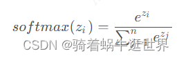
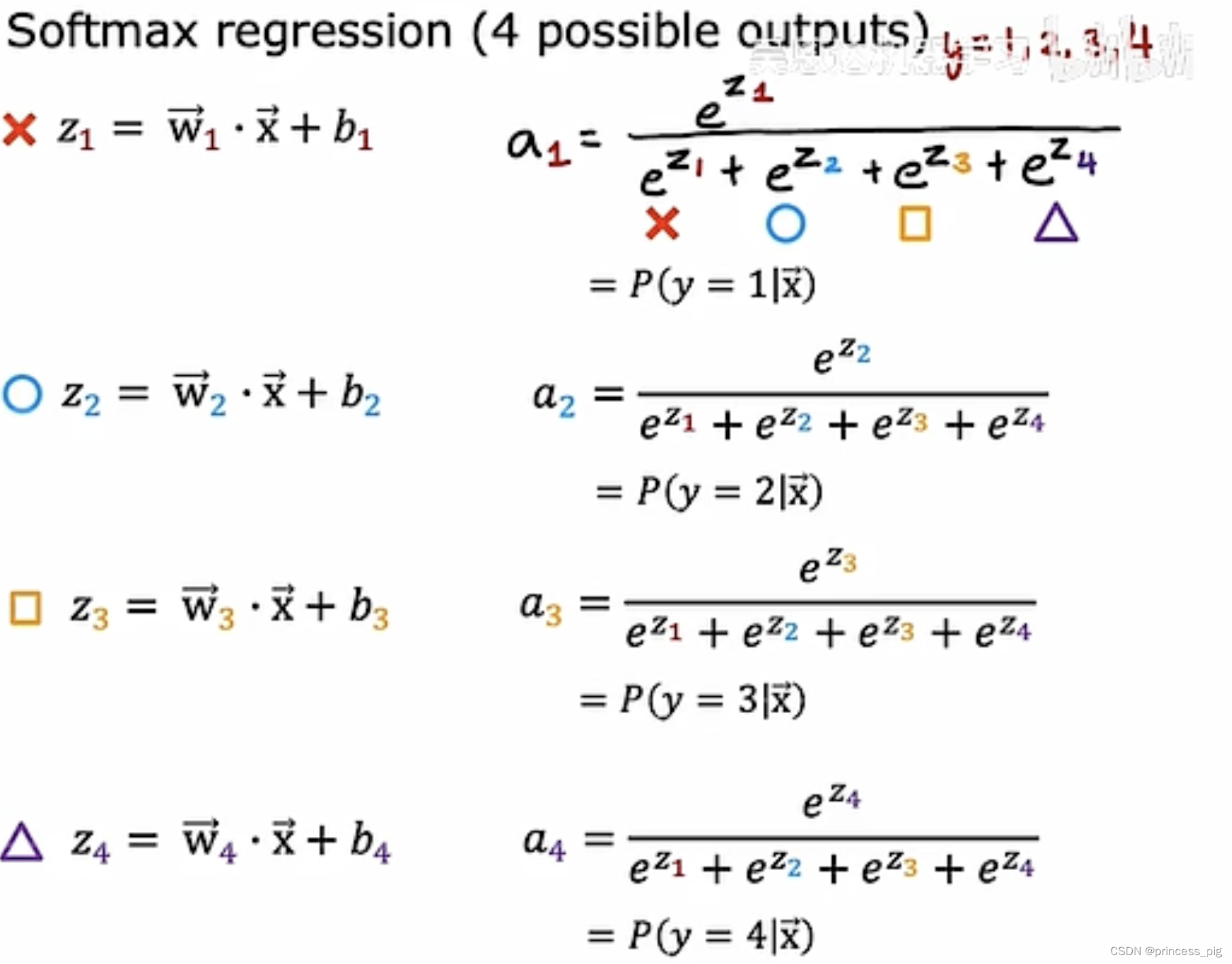
Softmax是神经网络中常用的一种激活函数,用于多分类任务。Softmax函数将未归一化的logits转换为概率分布。公式如下:
P ( y i ) = e z i ∑ j = 1 N e z j P(y_i) = \frac{e^{z_i}}{\sum_{j=1}^{N} e^{z_j}} P(yi)=∑j=1Nezjezi
其中, z i z_i zi是类别 i i i的logit, N N N是类别总数。
在大型词汇表情况下,计算Softmax需要对每个词的logit进行指数运算并归一化,这会导致计算成本随词汇表大小线性增长。因此,当词汇表非常大时,计算Softmax的代价非常高。
层次Softmax
层次Softmax(Hierarchical Softmax)是一种通过树结构来加速Softmax计算的方法。它将词汇表组织成一个树结构,每个叶节点代表一个词,每个内部节点代表一个路径选择的二分类器。通过这种方式,可以将计算复杂度从O(N)降低到O(log(N))。
层次Softmax的详细步骤
构建层次结构:
- 将词汇表组织成一棵二叉树或霍夫曼树。霍夫曼树可以根据词频来构建,使得高频词的路径更短,从而进一步加速计算。
路径表示:
- 对于每个词,通过树从根节点到叶节点的路径来表示。例如,假设词“banana”的路径为[根 -> 右 -> 左]。
路径概率计算:
- 每个内部节点都有一个二分类器,计算左子节点或右子节点的概率。
- 目标词的概率是从根节点到该词的路径上所有内部节点概率的乘积。
对于目标词 w w w,其概率表示为:
P ( w ∣ c o n t e x t ) = ∏ n ∈ p a t h ( w ) P ( n ∣ c o n t e x t ) P(w|context) = \prod_{n \in path(w)} P(n|context) P(w∣context)=n∈path(w)∏P(n∣context)
其中, p a t h ( w ) path(w) path(w)表示从根节点到词 w w w的路径上的所有内部节点。
训练过程:
- 使用负对数似然损失函数进行优化。
- 对于每个训练样本,计算从根节点到目标词的路径上的所有内部节点的概率,并根据实际路径更新模型参数。
对比分析
| 特点 | Softmax | 层次Softmax |
|---|---|---|
| 计算复杂度 | O(N) | O(log(N)) |
| 适用场景 | 小型词汇表 | 大型词汇表 |
| 实现复杂度 | 简单 | 复杂,需要构建树结构 |
| 计算效率 | 随词汇表大小增加而增加 | 随词汇表大小增加,增长较慢 |
为了更详细地展示层次Softmax与传统Softmax的对比,并包括实际数据和计算过程,下面我们使用一个简化的例子来说明。
案例说明 - 词汇表及其层次结构
假设我们有以下词汇表(词汇频率为假定):
| 词汇 | 频率 |
|---|---|
| apple | 7 |
| banana | 2 |
| cherry | 4 |
| date | 1 |
根据词汇频率,我们构建如下霍夫曼树:
       (*)
     /     \
  (apple)  (*)
           / \
      (cherry) (*)
               / \
         (banana) (date)
计算Softmax概率
假设在某个上下文下,模型输出以下logits:
| 词汇 | Logit z z z |
|---|---|
| apple | 1.5 |
| banana | 0.5 |
| cherry | 1.0 |
| date | 0.2 |
Softmax计算步骤:
- 计算每个词的指数:
e 1.5 = 4.4817 e^{1.5} = 4.4817 e1.5=4.4817
e 0.5 = 1.6487 e^{0.5} = 1.6487 e0.5=1.6487
e 1.0 = 2.7183 e^{1.0} = 2.7183 e1.0=2.7183
e 0.2 = 1.2214 e^{0.2} = 1.2214 e0.2=1.2214
- 计算所有指数的总和:
Z = 4.4817 + 1.6487 + 2.7183 + 1.2214 = 10.0701 Z = 4.4817 + 1.6487 + 2.7183 + 1.2214 = 10.0701 Z=4.4817+1.6487+2.7183+1.2214=10.0701
- 计算每个词的概率:
P ( a p p l e ) = 4.4817 10.0701 ≈ 0.445 P(apple) = \frac{4.4817}{10.0701} \approx 0.445 P(apple)=10.07014.4817≈0.445
P ( b a n a n a ) = 1.6487 10.0701 ≈ 0.164 P(banana) = \frac{1.6487}{10.0701} \approx 0.164 P(banana)=10.07011.6487≈0.164
P ( c h e r r y ) = 2.7183 10.0701 ≈ 0.270 P(cherry) = \frac{2.7183}{10.0701} \approx 0.270 P(cherry)=10.07012.7183≈0.270
P ( d a t e ) = 1.2214 10.0701 ≈ 0.121 P(date) = \frac{1.2214}{10.0701} \approx 0.121 P(date)=10.07011.2214≈0.121
计算层次Softmax概率
我们使用以下假设的特征向量和模型参数来计算每个内部节点的概率:
模型参数:
- 根节点二分类器:
- 权重 w r o o t = [ 0.5 , − 0.2 ] w_{root} = [0.5, -0.2] wroot=[0.5,−0.2]
- 偏置 b r o o t = 0 b_{root} = 0 broot=0
- 右子节点二分类器:
- 权重 w r i g h t = [ 0.3 , 0.4 ] w_{right} = [0.3, 0.4] wright=[0.3,0.4]
- 偏置 b r i g h t = − 0.1 b_{right} = -0.1 bright=−0.1
- 子树根二分类器:
- 权重 w s u b t r e e = [ − 0.4 , 0.2 ] w_{subtree} = [-0.4, 0.2] wsubtree=[−0.4,0.2]
- 偏置 b s u b t r e e = 0.2 b_{subtree} = 0.2 bsubtree=0.2
上下文特征向量:
- x c o n t e x t = [ 1 , 2 ] x_{context} = [1, 2] xcontext=[1,2]
1. 计算根节点概率
z r o o t = w r o o t ⋅ x c o n t e x t + b r o o t z_{root} = w_{root} \cdot x_{context} + b_{root} zroot=wroot⋅xcontext+broot
z r o o t = 0.5 × 1 + ( − 0.2 ) × 2 + 0 z_{root} = 0.5 \times 1 + (-0.2) \times 2 + 0 zroot=0.5×1+(−0.2)×2+0
z r o o t = 0.5 − 0.4 z_{root} = 0.5 - 0.4 zroot=0.5−0.4
z r o o t = 0.1 z_{root} = 0.1 zroot=0.1
使用sigmoid函数计算概率:
P ( l e f t ∣ c o n t e x t ) r o o t = σ ( z r o o t ) P(left|context)_{root} = \sigma(z_{root}) P(left∣context)root=σ(zroot)
P ( l e f t ∣ c o n t e x t ) r o o t = 1 1 + e − 0.1 P(left|context)_{root} = \frac{1}{1 + e^{-0.1}} P(left∣context)root=1+e−0.11
P ( l e f t ∣ c o n t e x t ) r o o t ≈ 1 1 + 0.9048 P(left|context)_{root} \approx \frac{1}{1 + 0.9048} P(left∣context)root≈1+0.90481
P ( l e f t ∣ c o n t e x t ) r o o t ≈ 0.525 P(left|context)_{root} \approx 0.525 P(left∣context)root≈0.525
P ( r i g h t ∣ c o n t e x t ) r o o t = 1 − P ( l e f t ∣ c o n t e x t ) r o o t P(right|context)_{root} = 1 - P(left|context)_{root} P(right∣context)root=1−P(left∣context)root
P ( r i g h t ∣ c o n t e x t ) r o o t = 1 − 0.525 P(right|context)_{root} = 1 - 0.525 P(right∣context)root=1−0.525
P ( r i g h t ∣ c o n t e x t ) r o o t ≈ 0.475 P(right|context)_{root} \approx 0.475 P(right∣context)root≈0.475
2. 计算右子节点概率
z r i g h t = w r i g h t ⋅ x c o n t e x t + b r i g h t z_{right} = w_{right} \cdot x_{context} + b_{right} zright=wright⋅xcontext+bright
z r i g h t = 0.3 × 1 + 0.4 × 2 − 0.1 z_{right} = 0.3 \times 1 + 0.4 \times 2 - 0.1 zright=0.3×1+0.4×2−0.1
z r i g h t = 0.3 + 0.8 − 0.1 z_{right} = 0.3 + 0.8 - 0.1 zright=0.3+0.8−0.1
z r i g h t = 1.0 z_{right} = 1.0 zright=1.0
使用sigmoid函数计算概率:
P ( l e f t ∣ c o n t e x t ) r i g h t = σ ( z r i g h t ) P(left|context)_{right} = \sigma(z_{right}) P(left∣context)right=σ(zright)
P ( l e f t ∣ c o n t e x t ) r i g h t = 1 1 + e − 1.0 P(left|context)_{right} = \frac{1}{1 + e^{-1.0}} P(left∣context)right=1+e−1.01
P ( l e f t ∣ c o n t e x t ) r i g h t ≈ 1 1 + 0.3679 P(left|context)_{right} \approx \frac{1}{1 + 0.3679} P(left∣context)right≈1+0.36791
P ( l e f t ∣ c o n t e x t ) r i g h t ≈ 0.731 P(left|context)_{right} \approx 0.731 P(left∣context)right≈0.731
P ( r i g h t ∣ c o n t e x t ) r i g h t = 1 − P ( l e f t ∣ c o n t e x t ) r i g h t P(right|context)_{right} = 1 - P(left|context)_{right} P(right∣context)right=1−P(left∣context)right
P ( r i g h t ∣ c o n t e x t ) r i g h t = 1 − 0.731 P(right|context)_{right} = 1 - 0.731 P(right∣context)right=1−0.731
P ( r i g h t ∣ c o n t e x t ) r i g h t ≈ 0.269 P(right|context)_{right} \approx 0.269 P(right∣context)right≈0.269
3. 计算子树根节点概率
z s u b t r e e = w s u b t r e e ⋅ x c o n t e x t + b s u b t r e e z_{subtree} = w_{subtree} \cdot x_{context} + b_{subtree} zsubtree=wsubtree⋅xcontext+bsubtree
z s u b t r e e = − 0.4 × 1 + 0.2 × 2 + 0.2 z_{subtree} = -0.4 \times 1 + 0.2 \times 2 + 0.2 zsubtree=−0.4×1+0.2×2+0.2
z s u b t r e e = − 0.4 + 0.4 + 0.2 z_{subtree} = -0.4 + 0.4 + 0.2 zsubtree=−0.4+0.4+0.2
z s u b t r e e = 0.2 z_{subtree} = 0.2 zsubtree=0.2
使用sigmoid函数计算概率:
P ( l e f t ∣ c o n t e x t ) s u b t r e e = σ ( z s u b t r e e ) P(left|context)_{subtree} = \sigma(z_{subtree}) P(left∣context)subtree=σ(zsubtree)
P ( l e f t ∣ c o n t e x t ) s u b t r e e = 1 1 + e − 0.2 P(left|context)_{subtree} = \frac{1}{1 + e^{-0.2}} P(left∣context)subtree=1+e−0.21
P ( l e f t ∣ c o n t e x t ) s u b t r e e ≈ 1 1 + 0.8187 P(left|context)_{subtree} \approx \frac{1}{1 + 0.8187} P(left∣context)subtree≈1+0.81871
P ( l e f t ∣ c o n t e x t ) s u b t r e e ≈ 0.55 P(left|context)_{subtree} \approx 0.55 P(left∣context)subtree≈0.55
P ( r i g h t ∣ c o n t e x t ) s u b t r e e = 1 − P ( l e f t ∣ c o n t e x t ) s u b t r e e P(right|context)_{subtree} = 1 - P(left|context)_{subtree} P(right∣context)subtree=1−P(left∣context)subtree
P ( r i g h t ∣ c o n t e x t ) s u b t r e e = 1 − 0.55 P(right|context)_{subtree} = 1 - 0.55 P(right∣context)subtree=1−0.55
P ( r i g h t ∣ c o n t e x t ) s u b t r e e ≈ 0.45 P(right|context)_{subtree} \approx 0.45 P(right∣context)subtree≈0.45
计算各个词的层次Softmax概率
1. apple
路径为[根 -> 左]
P ( a p p l e ) = P ( l e f t ∣ c o n t e x t ) r o o t ≈ 0.525 P(apple) = P(left|context)_{root} \approx 0.525 P(apple)=P(left∣context)root≈0.525
2. banana
路径为[根 -> 右 -> 右 -> 左]
P ( b a n a n a ) = P ( r i g h t ∣ c o n t e x t ) r o o t × P ( r i g h t ∣ c o n t e x t ) r i g h t × P ( l e f t ∣ c o n t e x t ) s u b t r e e P(banana) = P(right|context)_{root} \times P(right|context)_{right} \times P(left|context)_{subtree} P(banana)=P(right∣context)root×P(right∣context)right×P(left∣context)subtree
P ( b a n a n a ) ≈ 0.475 × 0.269 × 0.55 P(banana) \approx 0.475 \times 0.269 \times 0.55 P(banana)≈0.475×0.269×0.55
P ( b a n a n a ) ≈ 0.0702 P(banana) \approx 0.0702 P(banana)≈0.0702
3. cherry
路径为[根 -> 右 -> 左]
P ( c h e r r y ) = P ( r i g h t ∣ c o n t e x t ) r o o t × P ( l e f t ∣ c o n t e x t ) r i g h t P(cherry) = P(right|context)_{root} \times P(left|context)_{right} P(cherry)=P(right∣context)root×P(left∣context)right
P ( c h e r r y ) ≈ 0.475 × 0.731 P(cherry) \approx 0.475 \times 0.731 P(cherry)≈0.475×0.731
P ( c h e r r y ) ≈ 0.3472 P(cherry) \approx 0.3472 P(cherry)≈0.3472
4. date
路径为[根 -> 右 -> 右 -> 右]
P ( d a t e ) = P ( r i g h t ∣ c o n t e x t ) r o o t × P ( r i g h t ∣ c o n t e x t ) r i g h t × P ( r i g h t ∣ c o n t e x t ) s u b t r e e P(date) = P(right|context)_{root} \times P(right|context)_{right} \times P(right|context)_{subtree} P(date)=P(right∣context)root×P(right∣context)right×P(right∣context)subtree
P ( d a t e ) ≈ 0.475 × 0.269 × 0.45 P(date) \approx 0.475 \times 0.269 \times 0.45 P(date)≈0.475×0.269×0.45
P ( d a t e ) ≈ 0.0575 P(date) \approx 0.0575 P(date)≈0.0575
概率总结
| 词汇 | Softmax 概率 | 层次Softmax 概率 |
|---|---|---|
| apple | 0.445 | 0.525 |
| banana | 0.164 | 0.0702 |
| cherry | 0.270 | 0.3472 |
| date | 0.121 | 0.0575 |
以上结果显示了传统Softmax和层次Softmax的概率计算方法及其结果。通过构建霍夫曼树,层次Softmax显著减少了计算复杂度,特别适用于处理大规模词汇表的任务。
Softmax与层次Softmax总结
| 特点 | Softmax | 层次Softmax |
|---|---|---|
| 计算复杂度 | O(N) | O(log(N)) |
| 优点 | 简单直接,适用于小型词汇表 | 计算效率高,适用于大规模词汇表 |
| 缺点 | 计算量大,随着词汇表大小增加而线性增加 | 需要构建和维护层次结构,模型复杂性增加 |
| 适用场景 | 词汇表较小的多分类问题 | 词汇表非常大的自然语言处理任务,如语言建模和机器翻译 |
总结来说,层次Softmax通过树结构优化了大词汇表的概率计算,使其在处理大型词汇表的任务中具有显著优势,而传统Softmax则更适合小型词汇表的场景。


![==继承==下半部分机制详解[ C++ ]](https://i-blog.csdnimg.cn/direct/cfb743cdc7384804897b652cd74cbc77.png)