Python 机器学习 基础 之 算法链与管道 【通用的管道接口/网格搜索预处理步骤与模型参数/网格搜索选择使用哪个模型】的简单说明

Python 机器学习 基础 之 算法链与管道 【通用的管道接口/网格搜索预处理步骤与模型参数/网格搜索选择使用哪个模型】的简单说明

目录

Python 机器学习 基础 之 算法链与管道 【通用的管道接口/网格搜索预处理步骤与模型参数/网格搜索选择使用哪个模型】的简单说明

一、简单介绍

二、通用的管道接口

1、用make_pipeline 方便地创建管道

2、访问步骤属性

3、访问网格搜索管道中的属性

三、网格搜索预处理步骤与模型参数

四、网格搜索选择使用哪个模型

附录

一、参考文献

一、简单介绍

Python是一种跨平台的计算机程序设计语言。是一种面向对象的动态类型语言，最初被设计用于编写自动化脚本(shell)，随着版本的不断更新和语言新功能的添加，越多被用于独立的、大型项目的开发。Python是一种解释型脚本语言，可以应用于以下领域： Web 和 Internet开发、科学计算和统计、人工智能、教育、桌面界面开发、软件开发、后端开发、网络爬虫。

Python 机器学习是利用 Python 编程语言中的各种工具和库来实现机器学习算法和技术的过程。Python 是一种功能强大且易于学习和使用的编程语言，因此成为了机器学习领域的首选语言之一。Python 提供了丰富的机器学习库，如Scikit-learn、TensorFlow、Keras、PyTorch等，这些库包含了许多常用的机器学习算法和深度学习框架，使得开发者能够快速实现、测试和部署各种机器学习模型。

Python 机器学习涵盖了许多任务和技术，包括但不限于：

1. 监督学习：包括分类、回归等任务。
2. 无监督学习：如聚类、降维等。
3. 半监督学习：结合了有监督和无监督学习的技术。
4. 强化学习：通过与环境的交互学习来优化决策策略。
5. 深度学习：利用深度神经网络进行学习和预测。

通过 Python 进行机器学习，开发者可以利用其丰富的工具和库来处理数据、构建模型、评估模型性能，并将模型部署到实际应用中。Python 的易用性和庞大的社区支持使得机器学习在各个领域都得到了广泛的应用和发展。

二、通用的管道接口

Pipeline 类不但可用于预处理和分类，实际上还可以将任意数量的估计器连接在一起。

在机器学习中，使用管道（Pipeline）和算法链可以让数据预处理、特征选择和模型训练等步骤变得更加简洁和系统化。Scikit-learn 提供了一个通用的管道接口，通过 Pipeline 和 make_pipeline 来实现。这使得我们可以将多个步骤整合到一起，形成一个统一的工作流。下面是一些主要概念和如何使用通用的管道接口的详细说明。

定义

1. Pipeline:

   • Pipeline 是一个可以串联多个处理步骤的对象。每个步骤都是一个二元组，包含一个名字和一个估计器（如预处理步骤或模型）。
   • Pipeline 的最后一步必须是一个模型（如分类器或回归器），而中间步骤可以是任何数据转换器（如标准化、特征选择等）。

2. make_pipeline:

   • make_pipeline 是一个简化的工厂函数，用于创建一个 Pipeline 对象。它自动为每个步骤生成名称，无需手动指定名称。

共同点和区别

• 共同点:

  • 都可以将多个处理步骤整合到一起。
  • 都提供了统一的接口，可以像单个模型一样进行训练和预测。
  • 都支持超参数的网格搜索和交叉验证。

• 区别:

  • Pipeline 需要手动为每个步骤指定名称。
  • make_pipeline 自动为每个步骤生成名称，适合步骤较少且名称无关紧要的情况。

使用示例

1. 使用 Pipeline

from sklearn.pipeline import Pipeline
from sklearn.preprocessing import StandardScaler, PolynomialFeatures
from sklearn.linear_model import Ridge
from sklearn.model_selection import train_test_split
from sklearn.datasets import fetch_california_housing

# 加载数据
california = fetch_california_housing()
X_train, X_test, y_train, y_test = train_test_split(california.data, california.target, random_state=0)

# 创建管道
pipe = Pipeline([
    ('scaler', StandardScaler()),
    ('poly', PolynomialFeatures(degree=2)),
    ('ridge', Ridge())
])

# 训练模型
pipe.fit(X_train, y_train)

# 评估模型
train_score = pipe.score(X_train, y_train)
test_score = pipe.score(X_test, y_test)

print(f"Training score: {train_score:.2f}")
print(f"Test score: {test_score:.2f}")

1. 使用 make_pipeline

from sklearn.pipeline import make_pipeline

# 创建管道
pipe = make_pipeline(
    StandardScaler(),
    PolynomialFeatures(degree=2),
    Ridge()
)

# 训练模型
pipe.fit(X_train, y_train)

# 评估模型
train_score = pipe.score(X_train, y_train)
test_score = pipe.score(X_test, y_test)

print(f"Training score: {train_score:.2f}")
print(f"Test score: {test_score:.2f}")

选择和使用

• 选择:

  • 使用 Pipeline 当你希望显式地为每个步骤命名时。
  • 使用 make_pipeline 当步骤名称不重要或步骤较少时。

• 使用:

  • 管道允许你将数据预处理、特征生成和模型训练结合在一起，这样可以减少代码重复和错误。
  • 通过统一的接口，可以在整个数据处理和建模过程中保持一致性。
  • 可以将管道与 GridSearchCV 或 RandomizedSearchCV 结合使用，进行超参数调优。

例如，你可以构建一个包含特征提取、特征选择、缩放和分类的管道，总共有 4 个步骤。同样，最后一步可以用回归或聚类代替分类。

对于管道中估计器的唯一要求就是，除了最后一步之外的所有步骤都需要具有 transform 方法，这样它们可以生成新的数据表示，以供下一个步骤使用。

在调用 Pipeline.fit 的过程中，管道内部依次对每个步骤调用 fit 和 transform （或仅调用 fit_transform 。） ，其输入是前一个步骤中 transform 方法的输出。对于管道中的最后一步，则仅调用 fit 。

忽略某些细枝末节，其实现方法如下所示。请记住，pipeline.steps 是由元组组成的列表，所以 pipeline.steps[0][1] 是第一个估计器，pipeline.steps[1][1] 是第二个估计器，以此类推：

def fit(self, X, y):
    X_transformed = X
    for name, estimator in self.steps[:-1]:
        # 遍历除最后一步之外的所有步骤
        # 对数据进行拟合和变换
        X_transformed = estimator.fit_transform(X_transformed, y)
    # 对最后一步进行拟合
    self.steps[-1][1].fit(X_transformed, y)
    return self

使用 Pipeline 进行预测时，我们同样利用除最后一步之外的所有步骤对数据进行变换（transform ），然后对最后一步调用 predict ：

def predict(self, X):
    X_transformed = X
    for step in self.steps[:-1]:
        # 遍历除最后一步之外的所有步骤
        # 对数据进行变换
        X_transformed = step[1].transform(X_transformed)
    # 利用最后一步进行预测
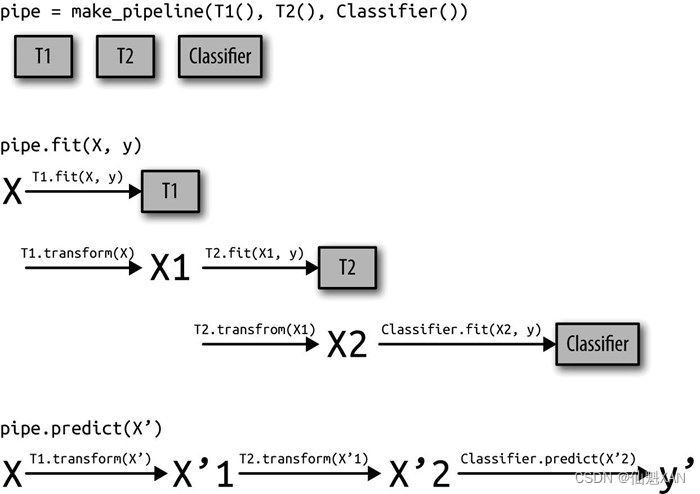
    return self.steps[-1][1].predict(X_transformed)

整个过程如图 6-3 所示，其中包含两个变换器（transformer）T1 和 T2 ，还有一个分类器（叫作 Classifier ）。

管道实际上比上图更加通用。管道的最后一步不需要具有 predict 函数，比如说，我们可以创建一个只包含一个缩放器和一个 PCA 的管道。由于最后一步（PCA ）具有 transform 方法，所以我们可以对管道调用 transform ，以得到将 PCA.transform 应用于前一个步骤处理过的数据后得到的输出。管道的最后一步只需要具有 fit 方法。

1、用make_pipeline 方便地创建管道

利用上述语法创建管道有时有点麻烦，我们通常不需要为每一个步骤提供用户指定的名称。有一个很方便的函数 make_pipeline ，可以为我们创建管道并根据每个步骤所属的类为其自动命名。make_pipeline 的语法如下所示：

from sklearn.pipeline import make_pipeline
from sklearn.pipeline import Pipeline
from sklearn.preprocessing import MinMaxScaler
from sklearn.svm import SVC

# 标准语法
pipe_long = Pipeline([("scaler", MinMaxScaler()), ("svm", SVC(C=100))])
# 缩写语法
pipe_short = make_pipeline(MinMaxScaler(), SVC(C=100))

管道对象 pipe_long 和 pipe_short 的作用完全相同，但 pipe_short 的步骤是自动命名的。我们可以通过查看 steps 属性来查看步骤的名称：

print("Pipeline steps:\n{}".format(pipe_short.steps))

Pipeline steps:
[('minmaxscaler', MinMaxScaler()), ('svc', SVC(C=100))]

这两个步骤被命名为 minmaxscaler 和 svc 。一般来说，步骤名称只是类名称的小写版本。如果多个步骤属于同一个类，则会附加一个数字：

from sklearn.preprocessing import StandardScaler
from sklearn.decomposition import PCA

pipe = make_pipeline(StandardScaler(), PCA(n_components=2), StandardScaler())
print("Pipeline steps:\n{}".format(pipe.steps))

Pipeline steps:
[('standardscaler-1', StandardScaler()), ('pca', PCA(n_components=2)), ('standardscaler-2', StandardScaler())]

如你所见，第一个 StandardScaler 步骤被命名为 standardscaler-1 ，而第二个被命名为 standardscaler-2 。但在这种情况下，使用具有明确名称的 Pipeline 构建可能更好，以便为每个步骤提供更具语义的名称。

2、访问步骤属性

通常来说，你希望检查管道中某一步骤的属性——比如线性模型的系数或 PCA 提取的成分。要想访问管道中的步骤，最简单的方法是通过 named_steps 属性，它是一个字典，将步骤名称映射为估计器：

from sklearn.datasets import load_breast_cancer

# 加载并划分数据
cancer = load_breast_cancer()

# 用前面定义的管道对cancer数据集进行拟合
pipe.fit(cancer.data)
# 从"pca"步骤中提取前两个主成分
components = pipe.named_steps["pca"].components_
print("components.shape: {}".format(components.shape))

components.shape: (2, 30)

3、访问网格搜索管道中的属性

本章前面说过，使用管道的主要原因之一就是进行网格搜索。一个常见的任务是在网格搜索内访问管道的某些步骤。我们对 cancer 数据集上的 LogisticRegression 分类器进行网格搜索，在将数据传入 LogisticRegression 分类器之前，先用 Pipeline 和 StandardScaler 对数据进行缩放。首先，我们用 make_pipeline 函数创建一个管道：

from sklearn.linear_model import LogisticRegression
pipe = make_pipeline(StandardScaler(), LogisticRegression())

接下来，我们创建一个参数网格。我们在第 2 章中说过，LogisticRegression 需要调节的正则化参数是参数 C 。我们对这个参数使用对数网格，在 0.01 和 100 之间进行搜索。由于我们使用了 make_pipeline 函数，所以管道中 LogisticRegression 步骤的名称是小写的类名称 logisticregression 。因此，为了调节参数 C ，我们必须指定 logisticregression__C 的参数网格：

param_grid = {'logisticregression__C': [0.01, 0.1, 1, 10, 100]}

像往常一样，我们将 cancer 数据集划分为训练集和测试集，并对网格搜索进行拟合：

from sklearn.model_selection import train_test_split
from sklearn.model_selection import GridSearchCV

X_train, X_test, y_train, y_test = train_test_split(
    cancer.data, cancer.target, random_state=4)
grid = GridSearchCV(pipe, param_grid, cv=5)
grid.fit(X_train, y_train)

那么我们如何访问 GridSearchCV 找到的最佳 LogisticRegression 模型的系数呢？我们从第 5 章中知道，GridSearchCV 找到的最佳模型（在所有训练数据上训练得到的模型）保存在 grid.best_estimator_ 中：

print("Best estimator:\n{}".format(grid.best_estimator_))

Best estimator:
Pipeline(steps=[('standardscaler', StandardScaler()),
                ('logisticregression', LogisticRegression(C=1))])

在我们的例子中，best_estimator_ 是一个管道，它包含两个步骤：standardscaler 和 logisticregression 。如前所述，我们可以使用管道的 named_steps 属性来访问 logisticregression 步骤：

print("Logistic regression step:\n{}".format(
      grid.best_estimator_.named_steps["logisticregression"]))

Logistic regression step:
LogisticRegression(C=1)

现在我们得到了训练过的 LogisticRegression 实例，下面我们可以访问与每个输入特征相关的系数（权重）：

print("Logistic regression coefficients:\n{}".format(
      grid.best_estimator_.named_steps["logisticregression"].coef_))

Logistic regression coefficients:
[[-0.4475566  -0.34609376 -0.41703843 -0.52889408 -0.15784407  0.60271339
  -0.71771325 -0.78367478  0.04847448  0.27478533 -1.29504052  0.05314385
  -0.69103766 -0.91925087 -0.14791795  0.46138699 -0.1264859  -0.10289486
   0.42812714  0.71492797 -1.08532414 -1.09273614 -0.85133685 -1.04104568
  -0.72839683  0.07656216 -0.83641023 -0.64928603 -0.6491432  -0.42968125]]

这个系数列表可能有点长，但它通常有助于理解你的模型。

三、网格搜索预处理步骤与模型参数

我们可以利用管道将机器学习工作流程中的所有处理步骤封装成一个 scikit-learn 估计器。这么做的另一个好处在于，现在我们可以使用监督任务（比如回归或分类）的输出来调节预处理参数 。在前几章里，我们在应用岭回归之前使用了 boston 数据集的多项式特征。下面我们用一个管道来重复这个建模过程。管道包含 3 个步骤：缩放数据、计算多项式特征与岭回归：

from sklearn.datasets import fetch_california_housing
from sklearn.model_selection import train_test_split
from sklearn.preprocessing import StandardScaler, PolynomialFeatures
from sklearn.linear_model import Ridge
from sklearn.pipeline import make_pipeline

# 加载加利福尼亚房价数据集
california = fetch_california_housing()
X_train, X_test, y_train, y_test = train_test_split(california.data, california.target,
                                                    random_state=0)

# 创建管道
pipe = make_pipeline(
    StandardScaler(),
    PolynomialFeatures(),
    Ridge())

我们怎么知道选择几次多项式，或者是否选择多项式或交互项呢？理想情况下，我们希望根据分类结果来选择 degree 参数。我们可以利用管道搜索 degree 参数以及 Ridge 的 alpha 参数。为了做到这一点，我们要定义一个包含这两个参数的 param_grid ，并用步骤名称作为前缀：

param_grid = {'polynomialfeatures__degree': [1, 2, 3],
              'ridge__alpha': [0.001, 0.01, 0.1, 1, 10, 100]}

现在我们可以再次运行网格搜索：

from sklearn.model_selection import GridSearchCV

grid = GridSearchCV(pipe, param_grid=param_grid, cv=5, n_jobs=-1)
grid.fit(X_train, y_train)

像之前所做的那样，我们可以用热图将交叉验证的结果可视化（见图 6-4）：

import matplotlib.pyplot as plt

plt.matshow(grid.cv_results_['mean_test_score'].reshape(3, -1),
            vmin=0, cmap="viridis")
plt.xlabel("ridge__alpha")
plt.ylabel("polynomialfeatures__degree")
plt.xticks(range(len(param_grid['ridge__alpha'])), param_grid['ridge__alpha'])
plt.yticks(range(len(param_grid['polynomialfeatures__degree'])),
           param_grid['polynomialfeatures__degree'])

plt.colorbar()

# plt.tight_layout()
plt.savefig('Images/05GridSearchPreprocessingStepsWithModelParameters-01.png', bbox_inches='tight')
plt.show()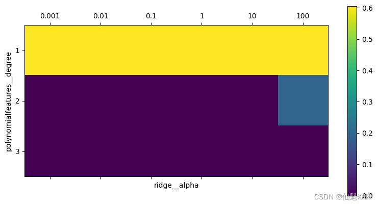

从交叉验证的结果中可以看出，使用二次多项式很有用，但三次多项式的效果比一次或二次都要差很多。从找到的最佳参数中也可以看出这一点：

print("Best parameters: {}".format(grid.best_params_))

Best parameters: {'polynomialfeatures__degree': 1, 'ridge__alpha': 10}

print("Test-set score: {:.2f}".format(grid.score(X_test, y_test)))

Test-set score: 0.59

为了对比，我们运行一个没有多项式特征的网格搜索：

param_grid = {'ridge__alpha': [0.001, 0.01, 0.1, 1, 10, 100]}
pipe = make_pipeline(StandardScaler(), Ridge())
grid = GridSearchCV(pipe, param_grid, cv=5)
grid.fit(X_train, y_train)
print("Score without poly features: {:.2f}".format(grid.score(X_test, y_test)))

Score without poly features: 0.59

正与我们观察图 6-4 中的网格搜索结果所预料的那样，不使用多项式特征得到了明显更差的结果。

同时搜索预处理参数与模型参数是一个非常强大的策略。但是要记住，GridSearchCV 会尝试指定参数的所有可能组合 。因此，向网格中添加更多参数，需要构建的模型数量将呈指数增长。

四、网格搜索选择使用哪个模型

你甚至可以进一步将 GridSearchCV 和 Pipeline 结合起来：还可以搜索管道中正在执行的实际步骤（比如用 StandardScaler 还是用 MinMaxScaler ）。这样会导致更大的搜索空间，应该予以仔细考虑。尝试所有可能的解决方案，通常并不是一种可行的机器学习策略。但下面是一个例子：在 iris 数据集上比较 RandomForestClassifier 和 SVC 。我们知道，SVC 可能需要对数据进行缩放，所以我们还需要搜索是使用 StandardScaler 还是不使用预处理。我们知道，RandomForestClassifier 不需要预处理。我们先定义管道。这里我们显式地对步骤命名。我们需要两个步骤，一个用于预处理，然后是一个分类器。我们可以用 SVC 和 StandardScaler 来将其实例化：

from sklearn.pipeline import Pipeline
from sklearn.preprocessing import StandardScaler
from sklearn.svm import SVC

pipe = Pipeline([('preprocessing', StandardScaler()), ('classifier', SVC())])

现在我们可以定义需要搜索的 parameter_grid 。我们希望 classifier 是 RandomForestClassifier 或 SVC 。由于这两种分类器需要调节不同的参数，并且需要不同的预处理，所以我们可以使用之前的“在非网格的空间中搜索”中所讲的搜索网格列表。为了将一个估计器分配给一个步骤，我们使用步骤名称作为参数名称。如果我们想跳过管道中的某个步骤（例如，RandomForest 不需要预处理），则可以将该步骤设置为 None ：

from sklearn.ensemble import RandomForestClassifier

param_grid = [
    {'classifier': [SVC()], 'preprocessing': [StandardScaler(), None],
     'classifier__gamma': [0.001, 0.01, 0.1, 1, 10, 100],
     'classifier__C': [0.001, 0.01, 0.1, 1, 10, 100]},
    {'classifier': [RandomForestClassifier(n_estimators=100)],
     'preprocessing': [None], 'classifier__max_features': [1, 2, 3]}]

现在，我们可以像前面一样将网格搜索实例化并在 cancer 数据集上运行：

from sklearn.model_selection import train_test_split
from sklearn.model_selection import GridSearchCV
from sklearn.datasets import load_breast_cancer

# 加载并划分数据
cancer = load_breast_cancer()

X_train, X_test, y_train, y_test = train_test_split(
    cancer.data, cancer.target, random_state=0)

grid = GridSearchCV(pipe, param_grid, cv=5)
grid.fit(X_train, y_train)

print("Best params:\n{}\n".format(grid.best_params_))
print("Best cross-validation score: {:.2f}".format(grid.best_score_))
print("Test-set score: {:.2f}".format(grid.score(X_test, y_test)))

Best params:
{'classifier': SVC(), 'classifier__C': 10, 'classifier__gamma': 0.01, 'preprocessing': StandardScaler()}

Best cross-validation score: 0.99
Test-set score: 0.98

网格搜索的结果是 SVC 与 StandardScaler 预处理，在 C=10 和 gamma=0.01 时给出最佳结果。

附录

一、参考文献

参考文献：[德] Andreas C. Müller [美] Sarah Guido 《Python Machine Learning Basics Tutorial》