白葡萄酒质量预测项目

注意：本文引用自专业人工智能社区Venus AI

更多AI知识请参考原站 （[www.aideeplearning.cn]）

项目背景

白葡萄酒是一种受欢迎的饮品，其质量受到广泛关注。了解和预测白葡萄酒的质量可以帮助酒厂和消费者做出更明智的选择。质量评估是一项复杂的任务，因为它受到多个化学特性的影响。因此，我们决定建立一个机器学习模型，以高精度预测白葡萄酒的质量。

项目目标

本项目的主要目标是构建一个能够高精度预测白葡萄酒质量的模型。通过使用白葡萄酒的化学特性数据，我们的模型将能够快速、准确地预测白葡萄酒的质量等级。这有助于酒厂改进酿造过程，确保生产高质量的葡萄酒。

项目应用

这个项目的应用非常广泛，一些潜在的应用包括：

1. 酒厂：酒厂可以使用这个模型来评估他们生产的葡萄酒的质量，并根据预测结果进行改进。
2. 消费者：消费者可以使用这个模型来选择适合他们口味的葡萄酒。
3. 餐馆和酒吧：餐馆和酒吧可以使用这个模型来选择他们的酒单中的葡萄酒。
4. 葡萄酒评审人：葡萄酒评审人可以使用这个模型来辅助他们的评价。

数据集描述

我们将使用的数据集包含了白葡萄酒的多个化学特性，以及每瓶葡萄酒的质量评级。以下是数据集中的主要特征：

• fixed acidity：固定酸度
• volatile acidity：挥发性酸度
• citric acid：柠檬酸含量
• residual sugar：残留糖分
• chlorides：氯化物含量
• free sulfur dioxide：游离二氧化硫含量
• total sulfur dioxide：总二氧化硫含量
• density：密度
• pH：pH值
• sulphates：硫酸盐含量
• alcohol：酒精含量
• quality：质量评级

模型选择与依赖库

为了预测白葡萄酒的质量，我们使用了以下机器学习模型进行训练和比较：

• K-最近邻算法（K-Nearest Neighbors）
• 决策树分类器（Decision Tree Classifier）
• 朴素贝叶斯（Naive Bayes）
• 随机森林分类器（Random Forest Classifier）
• 梯度提升分类器（Gradient Boosting Classifier）

依赖库

• numpy
• pandas
• matplotlib
• seaborn
• imblearn

评估指标

我们使用了以下评估指标来评估模型的性能：

• 混淆矩阵（confusion_matrix）
• 准确度（accuracy_score）
• 分类报告（classification_report）

代码实现

项目名称：白葡萄酒品质预测

问题陈述：

我们得到一个由白葡萄酒质量和决定葡萄酒质量的成分组成的数据集。 我们需要建立一个能够以最高精度预测葡萄酒质量的模型。

导入库并加载数据集

#导入库
import numpy as np
import pandas as pd
import matplotlib.pyplot as plt
import seaborn as sns
from imblearn.over_sampling import SMOTE

#加载数据集
white_wine_df = pd.read_csv("winequality-white.csv",sep=";")

white_wine_df.head()

	fixed acidity	volatile acidity	citric acid	residual sugar	chlorides	free sulfur dioxide	total sulfur dioxide	density	pH	sulphates	alcohol	quality
0	7.0	0.27	0.36	20.7	0.045	45.0	170.0	1.0010	3.00	0.45	8.8	6
1	6.3	0.30	0.34	1.6	0.049	14.0	132.0	0.9940	3.30	0.49	9.5	6
2	8.1	0.28	0.40	6.9	0.050	30.0	97.0	0.9951	3.26	0.44	10.1	6
3	7.2	0.23	0.32	8.5	0.058	47.0	186.0	0.9956	3.19	0.40	9.9	6
4	7.2	0.23	0.32	8.5	0.058	47.0	186.0	0.9956	3.19	0.40	9.9	6

white_wine_df.shape

(4898, 12)

white_wine_df.describe()

	fixed acidity	volatile acidity	citric acid	residual sugar	chlorides	free sulfur dioxide	total sulfur dioxide	density	pH	sulphates	alcohol	quality
count	4898.000000	4898.000000	4898.000000	4898.000000	4898.000000	4898.000000	4898.000000	4898.000000	4898.000000	4898.000000	4898.000000	4898.000000
mean	6.854788	0.278241	0.334192	6.391415	0.045772	35.308085	138.360657	0.994027	3.188267	0.489847	10.514267	5.877909
std	0.843868	0.100795	0.121020	5.072058	0.021848	17.007137	42.498065	0.002991	0.151001	0.114126	1.230621	0.885639
min	3.800000	0.080000	0.000000	0.600000	0.009000	2.000000	9.000000	0.987110	2.720000	0.220000	8.000000	3.000000
25%	6.300000	0.210000	0.270000	1.700000	0.036000	23.000000	108.000000	0.991723	3.090000	0.410000	9.500000	5.000000
50%	6.800000	0.260000	0.320000	5.200000	0.043000	34.000000	134.000000	0.993740	3.180000	0.470000	10.400000	6.000000
75%	7.300000	0.320000	0.390000	9.900000	0.050000	46.000000	167.000000	0.996100	3.280000	0.550000	11.400000	6.000000
max	14.200000	1.100000	1.660000	65.800000	0.346000	289.000000	440.000000	1.038980	3.820000	1.080000	14.200000	9.000000

# 总结数据集
white_wine_df.info()
<class 'pandas.core.frame.DataFrame'>
RangeIndex: 4898 entries, 0 to 4897
Data columns (total 12 columns):
 #   Column                Non-Null Count  Dtype  
---  ------                --------------  -----  
 0   fixed acidity         4898 non-null   float64
 1   volatile acidity      4898 non-null   float64
 2   citric acid           4898 non-null   float64
 3   residual sugar        4898 non-null   float64
 4   chlorides             4898 non-null   float64
 5   free sulfur dioxide   4898 non-null   float64
 6   total sulfur dioxide  4898 non-null   float64
 7   density               4898 non-null   float64
 8   pH                    4898 non-null   float64
 9   sulphates             4898 non-null   float64
 10  alcohol               4898 non-null   float64
 11  quality               4898 non-null   int64  
dtypes: float64(11), int64(1)
memory usage: 459.3 KB

#检查是否有空值
white_wine_df.isna().sum()

fixed acidity           0
volatile acidity        0
citric acid             0
residual sugar          0
chlorides               0
free sulfur dioxide     0
total sulfur dioxide    0
density                 0
pH                      0
sulphates               0
alcohol                 0
quality                 0
dtype: int64

不存在空值

探索性数据分析 (EDA)

白葡萄酒品质等级分布

white_wine_df['quality'].value_counts()

6    2198
5    1457
7     880
8     175
4     163
3      20
9       5
Name: quality, dtype: int64

• 我们拥有的大多数白葡萄酒数据都具有 5 到 7 之间的中等质量。

• 只有少数葡萄酒的品质非常高或非常低。

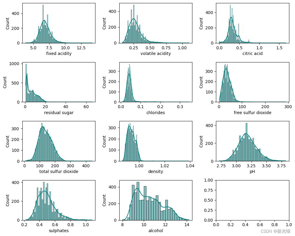
绘制独立特征的分布

import math

# Assuming the last column is not needed for plotting
num_features = len(white_wine_df.columns) - 1

# Calculate the number of rows and columns for the subplots
num_rows = math.ceil(num_features / 3)
fig, axes = plt.subplots(num_rows, 3, figsize=(10, 8))

i = 0
for row in range(num_rows):
    for col in range(3):
        if i < num_features:
            sns.histplot(white_wine_df[white_wine_df.columns[i]], ax=axes[row][col], color='teal', kde=True)
            i += 1

# Adjust layout
fig.tight_layout()

几乎所有分布图都遵循近似正态分布。

将葡萄酒的品质标记为低、中、高，并观察每种成分的浓度如何影响白葡萄酒的品质。

white_wine_df.head()

	fixed acidity	volatile acidity	citric acid	residual sugar	chlorides	free sulfur dioxide	total sulfur dioxide	density	pH	sulphates	alcohol	quality
0	7.0	0.27	0.36	20.7	0.045	45.0	170.0	1.0010	3.00	0.45	8.8	6
1	6.3	0.30	0.34	1.6	0.049	14.0	132.0	0.9940	3.30	0.49	9.5	6
2	8.1	0.28	0.40	6.9	0.050	30.0	97.0	0.9951	3.26	0.44	10.1	6
3	7.2	0.23	0.32	8.5	0.058	47.0	186.0	0.9956	3.19	0.40	9.9	6
4	7.2	0.23	0.32	8.5	0.058	47.0	186.0	0.9956	3.19	0.40	9.9	6

#标签编码
white_wine_df_new = white_wine_df.replace({'quality':{3:'low',4:'low',5:'medium',6:'medium',7:'medium',8:'high',9:'high'}})

white_wine_df_new.head()

	fixed acidity	volatile acidity	citric acid	residual sugar	chlorides	free sulfur dioxide	total sulfur dioxide	density	pH	sulphates	alcohol	quality
0	7.0	0.27	0.36	20.7	0.045	45.0	170.0	1.0010	3.00	0.45	8.8	medium
1	6.3	0.30	0.34	1.6	0.049	14.0	132.0	0.9940	3.30	0.49	9.5	medium
2	8.1	0.28	0.40	6.9	0.050	30.0	97.0	0.9951	3.26	0.44	10.1	medium
3	7.2	0.23	0.32	8.5	0.058	47.0	186.0	0.9956	3.19	0.40	9.9	medium
4	7.2	0.23	0.32	8.5	0.058	47.0	186.0	0.9956	3.19	0.40	9.9	medium

引入箱线图来根据质量观察葡萄酒成分的浓度。

# Get the columns to plot
columns_to_plot = white_wine_df_new.describe().columns

# Calculate the number of rows and columns for the subplot grid
n_cols = 3  # You can change this to fit your screen better
n_rows = (len(columns_to_plot) + n_cols - 1) // n_cols  # Calculate rows needed

# Create a figure and a grid of subplots
fig, axes = plt.subplots(n_rows, n_cols, figsize=(15, 5 * n_rows))

# Flatten the axes array for easy iteration
axes_flat = axes.flatten()

# Iterate over the columns and create a boxplot in each subplot
for i, col in enumerate(columns_to_plot):
    sns.boxplot(x='quality', y=col, data=white_wine_df_new, ax=axes_flat[i])

# Hide any unused subplots
for i in range(len(columns_to_plot), len(axes_flat)):
    axes_flat[i].set_visible(False)

# Adjust layout for better display
fig.tight_layout()

# Display the plot
plt.show()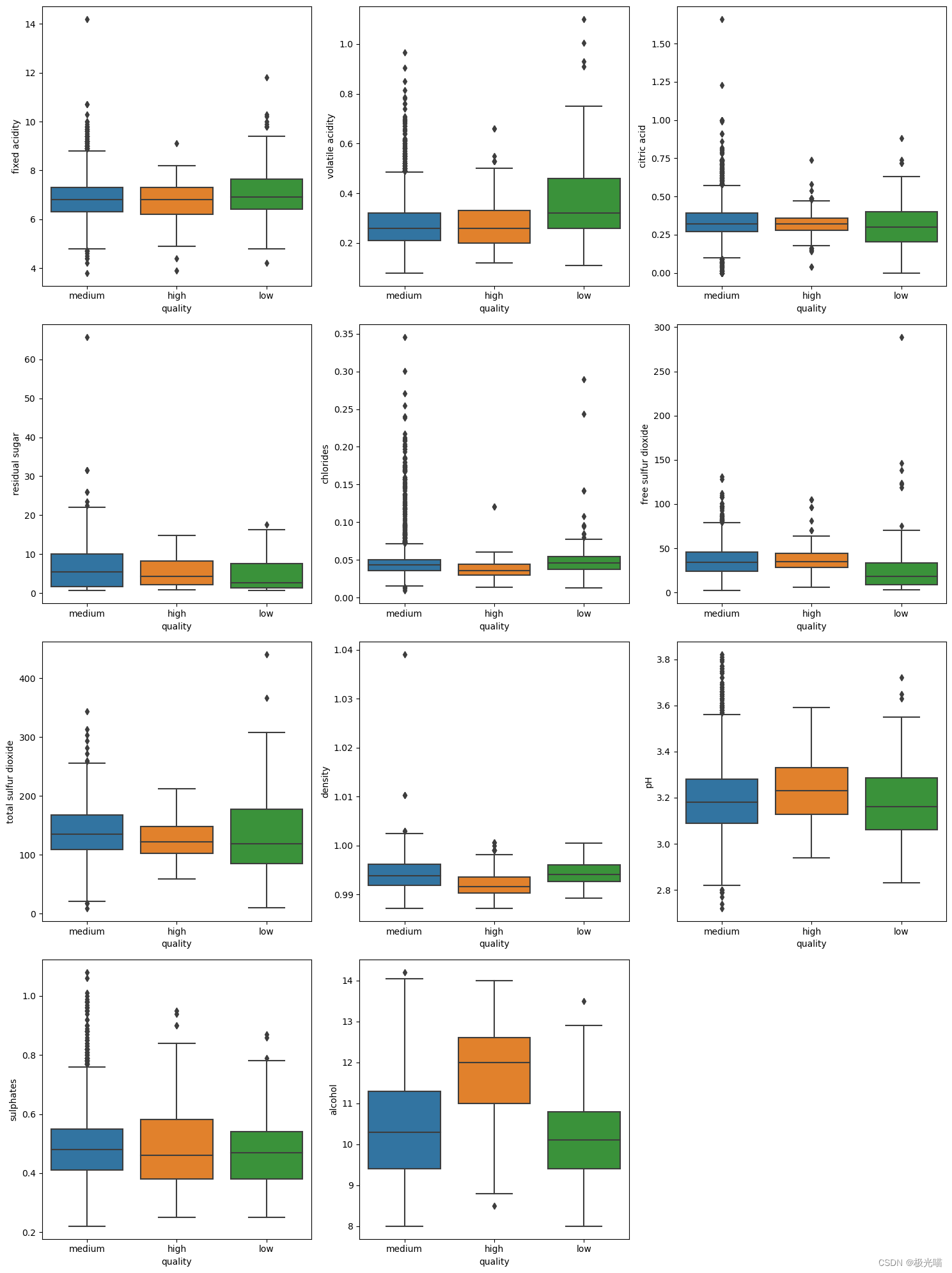

观察结果：

• 品质高的白葡萄酒，其酒精含量和pH值较高，而氯化物含量较低。
• 固定酸度和挥发酸度高的白葡萄酒质量较低。

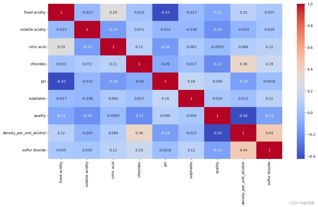
相关性

## 变量之间的相关性
plt.figure(figsize=(15,8))
correlation = white_wine_df.corr()
sns.heatmap((correlation), annot=True, cmap='coolwarm')

<Axes: >

观察：

• 观察到两个强相关数据

1. 密度v/s残糖
2. 密度v/s酒精

• 游离二氧化硫和总二氧化硫之间存在中等相关性。

• 密度与残糖呈正相关，同时我们还可以观察到，与非常低的残糖相比，密度对于葡萄酒的质量来说是更有价值的因素。这意味着我们可以删除残留糖特征来消除共线性。

• 密度与酒精呈负相关，但两者与质量具有良好的相关性。因此，删除它们中的任何一个都不是一个好的选择，而是我们可以将它们两者都引入来派生新的功能。

• 为了消除二氧化硫和总二氧化硫之间的共线性，我们将通过对它们求和来生成新特征二氧化硫。

# 消除多重共线性
white_wine_df.drop(columns='residual sugar',axis=1,inplace=True)
white_wine_df['density_per_unit_alcohol'] = white_wine_df['density']/white_wine_df['alcohol']
white_wine_df['sulfur dioxide'] = white_wine_df['free sulfur dioxide']+white_wine_df['total sulfur dioxide']

#删除原始列
white_wine_df.drop(columns=['free sulfur dioxide','total sulfur dioxide','density','alcohol'],axis=1,inplace=True)

white_wine_df.head()

	fixed acidity	volatile acidity	citric acid	chlorides	pH	sulphates	quality	density_per_unit_alcohol	sulfur dioxide
0	7.0	0.27	0.36	0.045	3.00	0.45	6	0.113750	215.0
1	6.3	0.30	0.34	0.049	3.30	0.49	6	0.104632	146.0
2	8.1	0.28	0.40	0.050	3.26	0.44	6	0.098525	127.0
3	7.2	0.23	0.32	0.058	3.19	0.40	6	0.100566	233.0
4	7.2	0.23	0.32	0.058	3.19	0.40	6	0.100566	233.0

## 变量之间的相关性
plt.figure(figsize=(15,8))
correlation = white_wine_df.corr()
sns.heatmap((correlation), annot=True, cmap='coolwarm')

<Axes: >

现在我们的数据没有显着的相关性。

数据预处理

#数据分割
X = white_wine_df[white_wine_df.columns.drop('quality')]
y = white_wine_df['quality']

y.value_counts()

6    2198
5    1457
7     880
8     175
4     163
3      20
9       5
Name: quality, dtype: int64

引入 SMOTE 来平衡数据

由于我们的数据严重不平衡，模型将无法在样本非常少的数据上进行学习，这最终会降低模型的准确性。因此，我们将使用一种称为“合成少数过采样技术”(SMOTE) 的技术来平衡我们的数据。

#使用 SMOTE 进行平衡
oversample = SMOTE(k_neighbors=4)
X,y = oversample.fit_resample(X,y)

y.value_counts()

6    2198
5    2198
7    2198
8    2198
4    2198
3    2198
9    2198
Name: quality, dtype: int64

数据现已平衡

训练-测试分开

#分为训练测试和扩展功能
from sklearn.preprocessing import MinMaxScaler
from sklearn.model_selection import train_test_split
X_train, X_test, y_train, y_test = train_test_split(X, y, test_size=0.2, random_state=1, stratify=y)
mmscaler = MinMaxScaler()
X_train = mmscaler.fit_transform(X_train)
X_test = mmscaler.transform(X_test)

模型选择

由于目标变量是具有多个类别的分类变量。我们需要应用一个适合多类分类的模型。

适用于该场景的模型有：

1. k-最近邻。 2.决策树分类器 3.朴素贝叶斯。 4.随机森林分类器
2. 梯度提升

注意：- 为了检测过度拟合，即未能通过模型​​概括模式，我们将为每个模型使用 k 倍交叉验证技术

1. k-最近邻

#使用 GridsearchCV 应用 k 折交叉验证并拟合模型。
from sklearn.model_selection import GridSearchCV
from sklearn.neighbors import KNeighborsClassifier
param_grid = {'n_neighbors': np.arange(1, 20,2)}
knn = KNeighborsClassifier()
knn_clf=KNeighborsClassifier()
knn_gscv = GridSearchCV(knn, param_grid,cv=5,return_train_score=True, verbose=1,scoring='accuracy')
knn_gscv.fit(X_train,y_train)
y_pred=knn_gscv.predict(X_test)

Fitting 5 folds for each of 10 candidates, totalling 50 fits

#评估模型
from sklearn.metrics import classification_report, confusion_matrix, accuracy_score
result = confusion_matrix(y_test, y_pred)
print(f"Confusion Matrix:\n{result}")
result1 = classification_report(y_test, y_pred)
print(f"Classification Report:\n{result1}")
result2 = accuracy_score(y_test,y_pred)
print(f"Accuracy:{round(result2,2)}\n\n")

Confusion Matrix:
[[440   0   0   0   0   0   0]
 [  3 417  13   3   3   1   0]
 [  2  23 324  56  27   7   0]
 [  4  23  71 260  58  24   0]
 [  2   9  11  44 338  35   1]
 [  0   0   0   7   5 428   0]
 [  0   0   0   0   0   0 439]]
Classification Report:
              precision    recall  f1-score   support

           3       0.98      1.00      0.99       440
           4       0.88      0.95      0.91       440
           5       0.77      0.74      0.76       439
           6       0.70      0.59      0.64       440
           7       0.78      0.77      0.78       440
           8       0.86      0.97      0.92       440
           9       1.00      1.00      1.00       439

    accuracy                           0.86      3078
   macro avg       0.85      0.86      0.86      3078
weighted avg       0.85      0.86      0.86      3078

Accuracy:0.86

2.决策树分类器

#使用 GridsearchCV 应用 k 折交叉验证并拟合模型。
from sklearn.model_selection import GridSearchCV
from sklearn.tree import DecisionTreeClassifier
param_grid = {'criterion':['gini','entropy'],'max_depth':[4,5,6,7,8,9,10,11,12,15,20,30,40,50,100]}
dt_clf=DecisionTreeClassifier()
dt_gscv = GridSearchCV(dt_clf, param_grid,cv=5,return_train_score=True, verbose=1,scoring='accuracy')
dt_gscv.fit(X_train,y_train)
y_pred=dt_gscv.predict(X_test)

Fitting 5 folds for each of 30 candidates, totalling 150 fits

dt_gscv.best_params_

{'criterion': 'gini', 'max_depth': 100}

#评估模型
from sklearn.metrics import classification_report, confusion_matrix, accuracy_score
result = confusion_matrix(y_test, y_pred)
print(f"Confusion Matrix:\n{result}")
result1 = classification_report(y_test, y_pred)
print(f"Classification Report:\n{result1}")
result2 = accuracy_score(y_test,y_pred)
print(f"Accuracy:{round(result2,2)}\n\n")

Confusion Matrix:
[[428   0   6   2   4   0   0]
 [  6 366  43  18   6   1   0]
 [  9  41 285  75  24   5   0]
 [  3  19  81 251  60  26   0]
 [  2   9  22  55 320  31   1]
 [  1   7   7  24  28 372   1]
 [  0   0   0   0   2   0 437]]
Classification Report:
              precision    recall  f1-score   support

           3       0.95      0.97      0.96       440
           4       0.83      0.83      0.83       440
           5       0.64      0.65      0.65       439
           6       0.59      0.57      0.58       440
           7       0.72      0.73      0.72       440
           8       0.86      0.85      0.85       440
           9       1.00      1.00      1.00       439

    accuracy                           0.80      3078
   macro avg       0.80      0.80      0.80      3078
weighted avg       0.80      0.80      0.80      3078

Accuracy:0.8

3.朴素贝叶斯

#使用 GridsearchCV 应用 k 折交叉验证并拟合模型。
from sklearn.model_selection import GridSearchCV
from sklearn.naive_bayes import GaussianNB
param_grid = {'var_smoothing': np.logspace(0,-9, num=100)}
gnb_clf = GaussianNB()
gnb_gscv = GridSearchCV(gnb_clf, param_grid,cv=5,return_train_score=True, verbose=1,scoring='accuracy')
gnb_gscv.fit(X_train,y_train)
y_pred=gnb_gscv.predict(X_test)

Fitting 5 folds for each of 100 candidates, totalling 500 fits

#评估模型
from sklearn.metrics import classification_report, confusion_matrix, accuracy_score
result = confusion_matrix(y_test, y_pred)
print(f"Confusion Matrix:\n{result}")
result1 = classification_report(y_test, y_pred)
print(f"Classification Report:\n{result1}")
result2 = accuracy_score(y_test,y_pred)
print(f"Accuracy:{round(result2,2)}\n\n")

Confusion Matrix:
[[237  16  67  13  70  10  27]
 [ 36 165 126  27  59  27   0]
 [ 26  44 234  37  85  12   1]
 [ 14  17 104  61 187  44  13]
 [  1   8  44  12 260  72  43]
 [  3   7  50  13 210 122  35]
 [  4   0   0   0   0  13 422]]
Classification Report:
              precision    recall  f1-score   support

           3       0.74      0.54      0.62       440
           4       0.64      0.38      0.47       440
           5       0.37      0.53      0.44       439
           6       0.37      0.14      0.20       440
           7       0.30      0.59      0.40       440
           8       0.41      0.28      0.33       440
           9       0.78      0.96      0.86       439

    accuracy                           0.49      3078
   macro avg       0.52      0.49      0.48      3078
weighted avg       0.52      0.49      0.48      3078

Accuracy:0.49

4.随机森林分类器

#使用 GridsearchCV 应用 k 折交叉验证并拟合模型。
from sklearn.model_selection import GridSearchCV
from sklearn.ensemble import RandomForestClassifier
param_grid = {'n_estimators':[100,200,500,1000], 'max_depth':[50,60,70,80,90,100]}
rf_clf=RandomForestClassifier()
rf_gscv = GridSearchCV(rf_clf, param_grid,cv=5,return_train_score=True, verbose=1,scoring='accuracy')
rf_gscv.fit(X_train,y_train)
y_pred=rf_gscv.predict(X_test)

rf_gscv.best_params_

{'max_depth': 60, 'n_estimators': 500}

#评估模型
from sklearn.metrics import classification_report, confusion_matrix, accuracy_score
result = confusion_matrix(y_test, y_pred)
print(f"Confusion Matrix:\n{result}")
result1 = classification_report(y_test, y_pred)
print(f"Classification Report:\n{result1}")
result2 = accuracy_score(y_test,y_pred)
print(f"Accuracy:{round(result2,2)}\n\n")

Confusion Matrix:
[[440   0   0   0   0   0   0]
 [  1 426   6   3   3   1   0]
 [  2  31 340  54  12   0   0]
 [  3   9  80 275  62  11   0]
 [  1   2  15  41 368  12   1]
 [  0   0   1   0   8 431   0]
 [  0   0   0   0   0   0 439]]
Classification Report:
              precision    recall  f1-score   support

           3       0.98      1.00      0.99       440
           4       0.91      0.97      0.94       440
           5       0.77      0.77      0.77       439
           6       0.74      0.62      0.68       440
           7       0.81      0.84      0.82       440
           8       0.95      0.98      0.96       440
           9       1.00      1.00      1.00       439

    accuracy                           0.88      3078
   macro avg       0.88      0.88      0.88      3078
weighted avg       0.88      0.88      0.88      3078

Accuracy:0.88

5.梯度提升模型

#使用 GridsearchCV 应用 k 折交叉验证并拟合模型。
from sklearn.model_selection import GridSearchCV
from sklearn.ensemble import GradientBoostingClassifier
param_grid = {
    "learning_rate": [0.01,0.05,0.1],
    "n_estimators":[50,100,500]
    }
gb_clf=GradientBoostingClassifier()
gb_gscv = GridSearchCV(gb_clf, param_grid,cv=5,return_train_score=True, verbose=2,scoring='accuracy')
gb_gscv.fit(X_train,y_train)
y_pred=gb_gscv.predict(X_test)

Fitting 5 folds for each of 9 candidates, totalling 45 fits
[CV] END ................learning_rate=0.01, n_estimators=50; total time=  11.1s
[CV] END ................learning_rate=0.01, n_estimators=50; total time=  12.0s
[CV] END ................learning_rate=0.01, n_estimators=50; total time=  11.0s
[CV] END ................learning_rate=0.01, n_estimators=50; total time=  11.0s
[CV] END ................learning_rate=0.01, n_estimators=50; total time=  11.0s
[CV] END ...............learning_rate=0.01, n_estimators=100; total time=  21.8s
[CV] END ...............learning_rate=0.01, n_estimators=100; total time=  21.8s
[CV] END ...............learning_rate=0.01, n_estimators=100; total time=  21.7s
[CV] END ...............learning_rate=0.01, n_estimators=100; total time=  21.9s
[CV] END ...............learning_rate=0.01, n_estimators=100; total time=  21.8s
[CV] END ...............learning_rate=0.01, n_estimators=500; total time= 1.8min
[CV] END ...............learning_rate=0.01, n_estimators=500; total time= 1.8min
[CV] END ...............learning_rate=0.01, n_estimators=500; total time= 1.8min
[CV] END ...............learning_rate=0.01, n_estimators=500; total time= 1.8min
[CV] END ...............learning_rate=0.01, n_estimators=500; total time= 1.8min
[CV] END ................learning_rate=0.05, n_estimators=50; total time=  10.9s
[CV] END ................learning_rate=0.05, n_estimators=50; total time=  10.9s
[CV] END ................learning_rate=0.05, n_estimators=50; total time=  10.9s
[CV] END ................learning_rate=0.05, n_estimators=50; total time=  11.0s
[CV] END ................learning_rate=0.05, n_estimators=50; total time=  10.9s
[CV] END ...............learning_rate=0.05, n_estimators=100; total time=  21.9s
[CV] END ...............learning_rate=0.05, n_estimators=100; total time=  21.9s
[CV] END ...............learning_rate=0.05, n_estimators=100; total time=  21.8s
[CV] END ...............learning_rate=0.05, n_estimators=100; total time=  22.7s
[CV] END ...............learning_rate=0.05, n_estimators=100; total time=  21.8s
[CV] END ...............learning_rate=0.05, n_estimators=500; total time= 1.8min
[CV] END ...............learning_rate=0.05, n_estimators=500; total time= 1.8min
[CV] END ...............learning_rate=0.05, n_estimators=500; total time= 1.8min
[CV] END ...............learning_rate=0.05, n_estimators=500; total time= 1.7min
[CV] END ...............learning_rate=0.05, n_estimators=500; total time= 1.7min
[CV] END .................learning_rate=0.1, n_estimators=50; total time=  10.3s
[CV] END .................learning_rate=0.1, n_estimators=50; total time=  10.3s
[CV] END .................learning_rate=0.1, n_estimators=50; total time=  10.2s
[CV] END .................learning_rate=0.1, n_estimators=50; total time=  10.8s
[CV] END .................learning_rate=0.1, n_estimators=50; total time=  10.4s
[CV] END ................learning_rate=0.1, n_estimators=100; total time=  20.5s
[CV] END ................learning_rate=0.1, n_estimators=100; total time=  20.4s
[CV] END ................learning_rate=0.1, n_estimators=100; total time=  20.3s
[CV] END ................learning_rate=0.1, n_estimators=100; total time=  20.4s
[CV] END ................learning_rate=0.1, n_estimators=500; total time= 1.7min
[CV] END ................learning_rate=0.1, n_estimators=500; total time= 1.7min
[CV] END ................learning_rate=0.1, n_estimators=500; total time= 1.7min
[CV] END ................learning_rate=0.1, n_estimators=500; total time= 1.7min
[CV] END ................learning_rate=0.1, n_estimators=500; total time= 1.7min

gb_gscv.best_params_

{'learning_rate': 0.1, 'n_estimators': 500}

#评估模型
from sklearn.metrics import classification_report, confusion_matrix, accuracy_score
result = confusion_matrix(y_test, y_pred)
print(f"Confusion Matrix:\n{result}")
result1 = classification_report(y_test, y_pred)
print(f"Classification Report:\n{result1}")
result2 = accuracy_score(y_test,y_pred)
print(f"Accuracy:{round(result2,2)}\n\n")

Confusion Matrix:
[[439   0   1   0   0   0   0]
 [  3 396  23  12   5   1   0]
 [  5  38 293  91  12   0   0]
 [  5   8  86 269  59  12   1]
 [  5  10  25  52 321  27   0]
 [  1   4   2   7  27 399   0]
 [  0   0   0   0   1   0 438]]
Classification Report:
              precision    recall  f1-score   support

           3       0.96      1.00      0.98       440
           4       0.87      0.90      0.88       440
           5       0.68      0.67      0.67       439
           6       0.62      0.61      0.62       440
           7       0.76      0.73      0.74       440
           8       0.91      0.91      0.91       440
           9       1.00      1.00      1.00       439

    accuracy                           0.83      3078
   macro avg       0.83      0.83      0.83      3078
weighted avg       0.83      0.83      0.83      3078

Accuracy:0.83

结论：

随机森林的模型精度最高，并且质量标签 5,6 和 7 的精度和召回率最高。 由于所有模型的质量标签 - 3、4、8、9 的精确度和召回率值都很高，因为它包含通过 SMOTE 技术创建的许多重复行来平衡数据，并且模型更容易记住重复的特征，导致高精度。

因此，质量标签的精度、召回率和 f1 分数- 5,6 和 7 非常重要，这对于模型随机森林来说是最高的。

因此我们得出结论，随机森林模型最适合我们的数据，准确度为 0.88。

代码与数据集下载

详情请见白葡萄酒质量预测项目-VenusAI (aideeplearning.cn)

结论

在我们的数据集上，随机森林分类器表现最佳，具有最高的准确度达到0.88，并且具有最佳的精确度和召回率值。这意味着我们的模型能够高度准确地预测白葡萄酒的质量评级，为酒厂和消费者提供了有用的信息。随机森林分类器是这个任务的最佳选择。