注意:本文引用自专业人工智能社区Venus AI
更多AI知识请参考原站 ([www.aideeplearning.cn])
在金融服务行业,贷款审批是一项关键任务,它不仅关系到资金的安全,还直接影响到金融机构的运营效率和风险管理。传统的审批流程往往依赖于人工审核,这不仅效率低下,而且容易受到主观判断的影响。为了解决这些问题,我们引入了一种基于机器学习的贷款预测模型,旨在提高贷款审批的准确性和效率。
项目背景
在当前的金融市场中,违约率的不断波动对贷款审批流程提出了新的挑战。传统方法往往无法有效预测和管理这些风险,因此需要一种更智能、更可靠的方法来评估贷款申请。通过使用机器学习,我们可以从大量历史数据中学习并识别违约的潜在风险,这不仅能提高贷款批准的准确性,还能大大降低金融机构的损失。
经过训练的模型将用于预测新的贷款申请是否有高风险。这将帮助金融机构在贷款批准过程中做出更加明智的决策,减少不良贷款的比例,提高整体的财务健康状况。
数据集
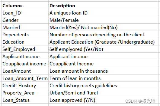
我们项目使用的数据集包括了广泛的客户特征,这些特征反映了贷款申请者的财务状况和背景。具体包括:
- 性别(Gender):申请人的性别。
- 婚姻状况(Married):申请人的婚姻状态。
- 受抚养人数(Dependents):申请人负责抚养的人数。
- 教育背景(Education):申请人的教育水平。
- 是否自雇(Self_Employed):申请人是否拥有自己的业务。
- 申请人收入(ApplicantIncome):申请人的月收入。
- 共同申请人收入(CoapplicantIncome):与申请人一同申请贷款的人的月收入。
- 贷款金额(LoanAmount):申请的贷款总额。
- 贷款期限(Loan_Amount_Term):预期的还款期限。
- 信用历史(Credit_History):申请人的信用记录。
- 财产区域(Property_Area):申请人财产所在的地理位置。
模型和依赖库
Models:
- RandomForestRegressor
- Decision Tree Regression
- logistic regression
Libraries:
- matplotlib==3.7.1
- numpy==1.24.3
- pandas==2.0.2
- scikit_learn==1.2.2
- seaborn==0.13.0
代码实现
金融贷款批准预测
项目背景
在金融领域,贷款审批是向任何人提供贷款之前需要执行的一项至关重要的任务。 这确保了批准的贷款将来可以收回。 然而,要确定一个人是否适合贷款或违约者,就很难确定有助于做出决定的性格和特征。
在这些情况下,使用机器学习的贷款预测模型成为非常有用的工具,可以根据过去的数据来预测该人是否违约。
我们获得了两个数据集(训练和测试),其中包含过去的交易,其中包括客户的一些特征以及显示客户是否违约的标签。 我们建立了一个模型,可以在训练数据集上执行,并可以预测贷款是否应获得批准。
About Data:
导入库并加载数据
#Impoting libraries
import pandas as pd
import numpy as np
import matplotlib.pyplot as plt
import seaborn as sns
df_train = pd.read_csv("train_u6lujuX_CVtuZ9i.csv")
df_test = pd.read_csv("test_Y3wMUE5_7gLdaTN.csv")df_train.head()| Loan_ID | Gender | Married | Dependents | Education | Self_Employed | ApplicantIncome | CoapplicantIncome | LoanAmount | Loan_Amount_Term | Credit_History | Property_Area | Loan_Status | |
|---|---|---|---|---|---|---|---|---|---|---|---|---|---|
| 0 | LP001002 | Male | No | 0 | Graduate | No | 5849 | 0.0 | NaN | 360.0 | 1.0 | Urban | Y |
| 1 | LP001003 | Male | Yes | 1 | Graduate | No | 4583 | 1508.0 | 128.0 | 360.0 | 1.0 | Rural | N |
| 2 | LP001005 | Male | Yes | 0 | Graduate | Yes | 3000 | 0.0 | 66.0 | 360.0 | 1.0 | Urban | Y |
| 3 | LP001006 | Male | Yes | 0 | Not Graduate | No | 2583 | 2358.0 | 120.0 | 360.0 | 1.0 | Urban | Y |
| 4 | LP001008 | Male | No | 0 | Graduate | No | 6000 | 0.0 | 141.0 | 360.0 | 1.0 | Urban | Y |
df_test.head()| Loan_ID | Gender | Married | Dependents | Education | Self_Employed | ApplicantIncome | CoapplicantIncome | LoanAmount | Loan_Amount_Term | Credit_History | Property_Area | |
|---|---|---|---|---|---|---|---|---|---|---|---|---|
| 0 | LP001015 | Male | Yes | 0 | Graduate | No | 5720 | 0 | 110.0 | 360.0 | 1.0 | Urban |
| 1 | LP001022 | Male | Yes | 1 | Graduate | No | 3076 | 1500 | 126.0 | 360.0 | 1.0 | Urban |
| 2 | LP001031 | Male | Yes | 2 | Graduate | No | 5000 | 1800 | 208.0 | 360.0 | 1.0 | Urban |
| 3 | LP001035 | Male | Yes | 2 | Graduate | No | 2340 | 2546 | 100.0 | 360.0 | NaN | Urban |
| 4 | LP001051 | Male | No | 0 | Not Graduate | No | 3276 | 0 | 78.0 | 360.0 | 1.0 | Urban |
#shape of data
df_train.shape
(614, 13)
#data summary
df_train.describe()| ApplicantIncome | CoapplicantIncome | LoanAmount | Loan_Amount_Term | Credit_History | |
|---|---|---|---|---|---|
| count | 614.000000 | 614.000000 | 592.000000 | 600.00000 | 564.000000 |
| mean | 5403.459283 | 1621.245798 | 146.412162 | 342.00000 | 0.842199 |
| std | 6109.041673 | 2926.248369 | 85.587325 | 65.12041 | 0.364878 |
| min | 150.000000 | 0.000000 | 9.000000 | 12.00000 | 0.000000 |
| 25% | 2877.500000 | 0.000000 | 100.000000 | 360.00000 | 1.000000 |
| 50% | 3812.500000 | 1188.500000 | 128.000000 | 360.00000 | 1.000000 |
| 75% | 5795.000000 | 2297.250000 | 168.000000 | 360.00000 | 1.000000 |
| max | 81000.000000 | 41667.000000 | 700.000000 | 480.00000 | 1.000000 |
df_train.info()<class 'pandas.core.frame.DataFrame'> RangeIndex: 614 entries, 0 to 613 Data columns (total 13 columns): # Column Non-Null Count Dtype --- ------ -------------- ----- 0 Loan_ID 614 non-null object 1 Gender 601 non-null object 2 Married 611 non-null object 3 Dependents 599 non-null object 4 Education 614 non-null object 5 Self_Employed 582 non-null object 6 ApplicantIncome 614 non-null int64 7 CoapplicantIncome 614 non-null float64 8 LoanAmount 592 non-null float64 9 Loan_Amount_Term 600 non-null float64 10 Credit_History 564 non-null float64 11 Property_Area 614 non-null object 12 Loan_Status 614 non-null object dtypes: float64(4), int64(1), object(8) memory usage: 62.5+ KB
数据清洗
# 检测空值
df_train.isna().sum()
Loan_ID 0 Gender 13 Married 3 Dependents 15 Education 0 Self_Employed 32 ApplicantIncome 0 CoapplicantIncome 0 LoanAmount 22 Loan_Amount_Term 14 Credit_History 50 Property_Area 0 Loan_Status 0 dtype: int64
有很多空值,Credit_History 的最大值为 50。
去除所有空值
# Dropping all the null values
drop_list = ['Gender','Married','Dependents','Self_Employed','LoanAmount','Loan_Amount_Term','Credit_History']
for col in drop_list:
df_train = df_train[~df_train[col].isna()]df_train.isna().sum()Loan_ID 0 Gender 0 Married 0 Dependents 0 Education 0 Self_Employed 0 ApplicantIncome 0 CoapplicantIncome 0 LoanAmount 0 Loan_Amount_Term 0 Credit_History 0 Property_Area 0 Loan_Status 0 dtype: int64
Loan_ID 列没用,这里删除它
# dropping Loan_ID
df_train.drop(columns='Loan_ID',axis=1, inplace=True)df_train.shape(480, 12)
#data summary
df_train.describe()| ApplicantIncome | CoapplicantIncome | LoanAmount | Loan_Amount_Term | Credit_History | |
|---|---|---|---|---|---|
| count | 480.000000 | 480.000000 | 480.000000 | 480.000000 | 480.000000 |
| mean | 5364.231250 | 1581.093583 | 144.735417 | 342.050000 | 0.854167 |
| std | 5668.251251 | 2617.692267 | 80.508164 | 65.212401 | 0.353307 |
| min | 150.000000 | 0.000000 | 9.000000 | 36.000000 | 0.000000 |
| 25% | 2898.750000 | 0.000000 | 100.000000 | 360.000000 | 1.000000 |
| 50% | 3859.000000 | 1084.500000 | 128.000000 | 360.000000 | 1.000000 |
| 75% | 5852.500000 | 2253.250000 | 170.000000 | 360.000000 | 1.000000 |
| max | 81000.000000 | 33837.000000 | 600.000000 | 480.000000 | 1.000000 |
数据分析(EDA)
df_train.head()| Gender | Married | Dependents | Education | Self_Employed | ApplicantIncome | CoapplicantIncome | LoanAmount | Loan_Amount_Term | Credit_History | Property_Area | Loan_Status | |
|---|---|---|---|---|---|---|---|---|---|---|---|---|
| 1 | Male | Yes | 1 | Graduate | No | 4583 | 1508.0 | 128.0 | 360.0 | 1.0 | Rural | N |
| 2 | Male | Yes | 0 | Graduate | Yes | 3000 | 0.0 | 66.0 | 360.0 | 1.0 | Urban | Y |
| 3 | Male | Yes | 0 | Not Graduate | No | 2583 | 2358.0 | 120.0 | 360.0 | 1.0 | Urban | Y |
| 4 | Male | No | 0 | Graduate | No | 6000 | 0.0 | 141.0 | 360.0 | 1.0 | Urban | Y |
| 5 | Male | Yes | 2 | Graduate | Yes | 5417 | 4196.0 | 267.0 | 360.0 | 1.0 | Urban | Y |
#distribution of Churn data
sns.displot(data=df_train,x='Loan_Status')
<seaborn.axisgrid.FacetGrid at 0x1f54d853bb0>
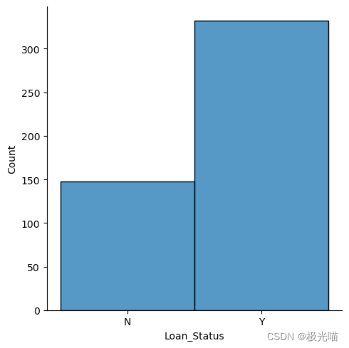
数据集是不平衡的,但是不是非常严重
自变量相对于因变量的分布.
# 设置分类特征
categorical_features=list(df_train.columns)
numeical_features = list(df_train.describe().columns)
for elem in numeical_features:
 categorical_features.remove(elem)
categorical_features = categorical_features[:-1]
categorical_features
['Gender', 'Married', 'Dependents', 'Education', 'Self_Employed', 'Property_Area']
# Set categorical and numerical features
categorical_features = list(df_train.columns)
numerical_features = list(df_train.describe().columns)
for elem in numerical_features:
    categorical_features.remove(elem)
categorical_features.remove('Loan_Status')  # Assuming 'Loan_Status' is not a feature to plot

# Determine the layout of subplots
n_cols = 2  # Can be adjusted based on preference
n_rows = (len(categorical_features) + 1) // n_cols

# Create a grid of subplots
fig, axes = plt.subplots(nrows=n_rows, ncols=n_cols, figsize=(12, n_rows * 4))

# Flatten the axes array for easy iteration
axes = axes.flatten()

# Plot each bar chart
for i, col in enumerate(categorical_features):
    df_train.groupby([col, 'Loan_Status']).size().unstack().plot(kind='bar', stacked=True, ax=axes[i])
    axes[i].set_title(f'Total count of Loan_Status grouped by {col}')
    axes[i].set_ylabel('Count')

# Adjust layout and display the plot
plt.tight_layout()
plt.show()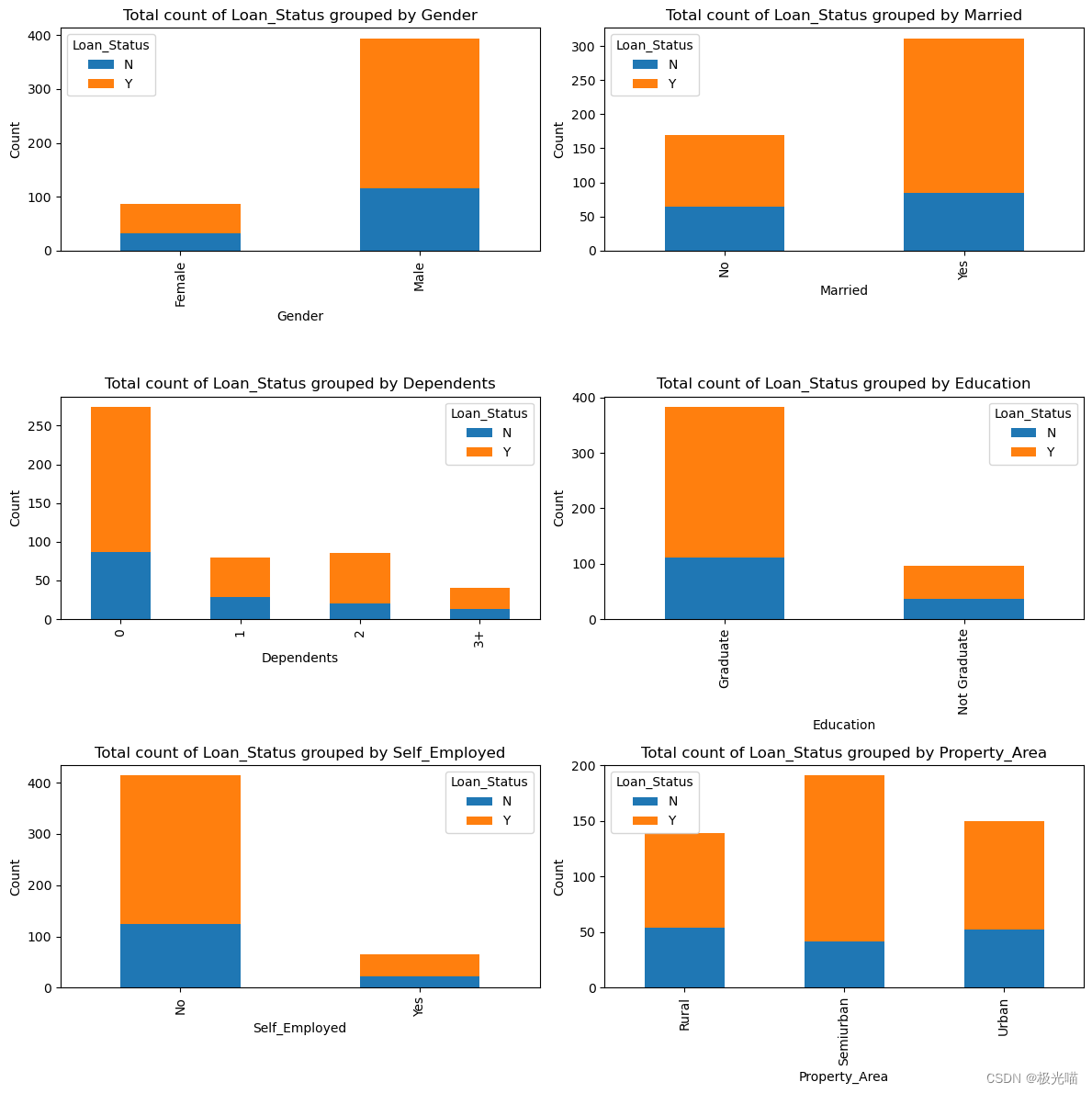
从上面的图中观察到的结果:
- 与女性相比,男性获得贷款批准的比例更高。
与非毕业生相比,贷款审批对毕业生更有利。
与受雇者相比,个体经营者获得贷款批准的机会较少。
- 城乡结合部的贷款批准率最高。
让我们看看按因变量分组的连续自变量
numerical_features = df_train.describe().columns

# Determine the layout of subplots
n_cols = 2  # Adjust based on preference
n_rows = (len(numerical_features) + 1) // n_cols

# Create a grid of subplots
fig, axes = plt.subplots(nrows=n_rows, ncols=n_cols, figsize=(12, n_rows * 4))

# Flatten the axes array for easy iteration
axes = axes.flatten()

# Plot each boxplot
for i, col in enumerate(numerical_features):
    sns.boxplot(x='Loan_Status', y=col, data=df_train, ax=axes[i])
    axes[i].set_title(f'Distribution of {col} grouped by Loan_Status')

# Adjust layout and display the plot
plt.tight_layout()
plt.show()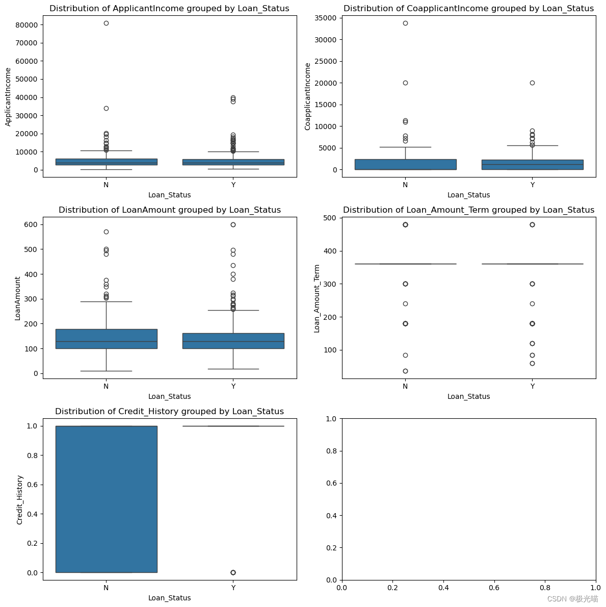
我们可以在数据中观察到很多异常值。
从上面的箱线图中无法得出任何正确的结论。
相关性分析
 ## Correlation between variables
plt.figure(figsize=(15,8))
correlation = df_train.corr()
sns.heatmap((correlation), annot=True, cmap='coolwarm')
<Axes: >

没有观察到任何显着的相关性。
数据预处理
df_train.head()| Gender | Married | Dependents | Education | Self_Employed | ApplicantIncome | CoapplicantIncome | LoanAmount | Loan_Amount_Term | Credit_History | Property_Area | Loan_Status | |
|---|---|---|---|---|---|---|---|---|---|---|---|---|
| 1 | Male | Yes | 1 | Graduate | No | 4583 | 1508.0 | 128.0 | 360.0 | 1.0 | Rural | N |
| 2 | Male | Yes | 0 | Graduate | Yes | 3000 | 0.0 | 66.0 | 360.0 | 1.0 | Urban | Y |
| 3 | Male | Yes | 0 | Not Graduate | No | 2583 | 2358.0 | 120.0 | 360.0 | 1.0 | Urban | Y |
| 4 | Male | No | 0 | Graduate | No | 6000 | 0.0 | 141.0 | 360.0 | 1.0 | Urban | Y |
| 5 | Male | Yes | 2 | Graduate | Yes | 5417 | 4196.0 | 267.0 | 360.0 | 1.0 | Urban | Y |
df_train['Property_Area'].value_counts()Semiurban 191 Urban 150 Rural 139 Name: Property_Area, dtype: int64
df_train['Credit_History'].value_counts()1.0 410 0.0 70 Name: Credit_History, dtype: int64
df_train['Dependents'].value_counts()0 274 2 85 1 80 3+ 41 Name: Dependents, dtype: int64
使用标签编码将分类列转换为数字
#Label encoding for some categorical features
df_train_new = df_train.copy()
label_col_list = ['Married','Self_Employed']
for col in label_col_list:
  df_train_new=df_train_new.replace({col:{'Yes':1,'No':0}})
df_train_new=df_train_new.replace({'Gender':{'Male':1,'Female':0}})
df_train_new=df_train_new.replace({'Education':{'Graduate':1,'Not Graduate':0}})
df_train_new=df_train_new.replace({'Loan_Status':{'Y':1,'N':0}})对于其余的分类特征,我们将进行一种热编码:
#one hot encoding
df_train_new = pd.get_dummies(df_train_new, columns=["Dependents","Property_Area"])df_train_new.head()| Gender | Married | Education | Self_Employed | ApplicantIncome | CoapplicantIncome | LoanAmount | Loan_Amount_Term | Credit_History | Loan_Status | Dependents_0 | Dependents_1 | Dependents_2 | Dependents_3+ | Property_Area_Rural | Property_Area_Semiurban | Property_Area_Urban | |
|---|---|---|---|---|---|---|---|---|---|---|---|---|---|---|---|---|---|
| 1 | 1 | 1 | 1 | 0 | 4583 | 1508.0 | 128.0 | 360.0 | 1.0 | 0 | 0 | 1 | 0 | 0 | 1 | 0 | 0 |
| 2 | 1 | 1 | 1 | 1 | 3000 | 0.0 | 66.0 | 360.0 | 1.0 | 1 | 1 | 0 | 0 | 0 | 0 | 0 | 1 |
| 3 | 1 | 1 | 0 | 0 | 2583 | 2358.0 | 120.0 | 360.0 | 1.0 | 1 | 1 | 0 | 0 | 0 | 0 | 0 | 1 |
| 4 | 1 | 0 | 1 | 0 | 6000 | 0.0 | 141.0 | 360.0 | 1.0 | 1 | 1 | 0 | 0 | 0 | 0 | 0 | 1 |
| 5 | 1 | 1 | 1 | 1 | 5417 | 4196.0 | 267.0 | 360.0 | 1.0 | 1 | 0 | 0 | 1 | 0 | 0 | 0 | 1 |
标准化连续变量。
#standardize continuous features
from scipy.stats import zscore
df_train_new[['ApplicantIncome','CoapplicantIncome','LoanAmount','Loan_Amount_Term']]=df_train_new[['ApplicantIncome','CoapplicantIncome','LoanAmount','Loan_Amount_Term']].apply(zscore) df_train_new.head()| Gender | Married | Education | Self_Employed | ApplicantIncome | CoapplicantIncome | LoanAmount | Loan_Amount_Term | Credit_History | Loan_Status | Dependents_0 | Dependents_1 | Dependents_2 | Dependents_3+ | Property_Area_Rural | Property_Area_Semiurban | Property_Area_Urban | |
|---|---|---|---|---|---|---|---|---|---|---|---|---|---|---|---|---|---|
| 1 | 1 | 1 | 1 | 0 | -0.137970 | -0.027952 | -0.208089 | 0.275542 | 1.0 | 0 | 0 | 1 | 0 | 0 | 1 | 0 | 0 |
| 2 | 1 | 1 | 1 | 1 | -0.417536 | -0.604633 | -0.979001 | 0.275542 | 1.0 | 1 | 1 | 0 | 0 | 0 | 0 | 0 | 1 |
| 3 | 1 | 1 | 0 | 0 | -0.491180 | 0.297100 | -0.307562 | 0.275542 | 1.0 | 1 | 1 | 0 | 0 | 0 | 0 | 0 | 1 |
| 4 | 1 | 0 | 1 | 0 | 0.112280 | -0.604633 | -0.046446 | 0.275542 | 1.0 | 1 | 1 | 0 | 0 | 0 | 0 | 0 | 1 |
| 5 | 1 | 1 | 1 | 1 | 0.009319 | 0.999978 | 1.520245 | 0.275542 | 1.0 | 1 | 0 | 0 | 1 | 0 | 0 | 0 | 1 |
# Repositioning the dependent variable to last index
last_column = df_train_new.pop('Loan_Status')
df_train_new.insert(16, 'Loan_Status', last_column)
df_train_new.head()| Gender | Married | Education | Self_Employed | ApplicantIncome | CoapplicantIncome | LoanAmount | Loan_Amount_Term | Credit_History | Dependents_0 | Dependents_1 | Dependents_2 | Dependents_3+ | Property_Area_Rural | Property_Area_Semiurban | Property_Area_Urban | Loan_Status | |
|---|---|---|---|---|---|---|---|---|---|---|---|---|---|---|---|---|---|
| 1 | 1 | 1 | 1 | 0 | -0.137970 | -0.027952 | -0.208089 | 0.275542 | 1.0 | 0 | 1 | 0 | 0 | 1 | 0 | 0 | 0 |
| 2 | 1 | 1 | 1 | 1 | -0.417536 | -0.604633 | -0.979001 | 0.275542 | 1.0 | 1 | 0 | 0 | 0 | 0 | 0 | 1 | 1 |
| 3 | 1 | 1 | 0 | 0 | -0.491180 | 0.297100 | -0.307562 | 0.275542 | 1.0 | 1 | 0 | 0 | 0 | 0 | 0 | 1 | 1 |
| 4 | 1 | 0 | 1 | 0 | 0.112280 | -0.604633 | -0.046446 | 0.275542 | 1.0 | 1 | 0 | 0 | 0 | 0 | 0 | 1 | 1 |
| 5 | 1 | 1 | 1 | 1 | 0.009319 | 0.999978 | 1.520245 | 0.275542 | 1.0 | 0 | 0 | 1 | 0 | 0 | 0 | 1 | 1 |
数据处理完毕,准备训练模型
数据集划分
由于我们的数据仅用于训练,其他数据可用于测试。 我们仍然会进行训练测试分割,因为测试数据没有标记,并且有必要根据未见过的数据评估模型。
X= df_train_new.iloc[:,:-1]
y= df_train_new.iloc[:,-1]
from sklearn.model_selection import train_test_split
X_train, X_test, y_train, y_test = train_test_split( X,y , test_size = 0.2, random_state = 0)
print(X_train.shape)
print(X_test.shape)
(384, 16) (96, 16)
y_train.value_counts()1 271 0 113 Name: Loan_Status, dtype: int64
y_test.value_counts()1 61 0 35 Name: Loan_Status, dtype: int64
对训练数据进行逻辑回归拟合
#Importing and fitting Logistic regression
from sklearn.linear_model import LogisticRegression

lr = LogisticRegression(fit_intercept=True, max_iter=10000,random_state=0)
lr.fit(X_train, y_train)
LogisticRegression
LogisticRegression(max_iter=10000, random_state=0)
# Get the model coefficients
lr.coef_
array([[ 0.23272114, 0.57128602, 0.26384918, -0.24617035, 0.15924191,
-0.14703758, -0.19280038, -0.16392914, 2.97399665, -0.18202629,
-0.27741114, 0.17256535, 0.28601466, -0.30275813, 0.64592912,
-0.3440284 ]])
#model intercept
lr.intercept_
array([-2.1943974])
评价训练模型的性能
# Get the predicted probabilities
train_preds = lr.predict_proba(X_train)
test_preds = lr.predict_proba(X_test)test_predsarray([[0.23916396, 0.76083604],
[0.24506751, 0.75493249],
[0.04933527, 0.95066473],
[0.20146124, 0.79853876],
[0.2347122 , 0.7652878 ],
[0.05817427, 0.94182573],
[0.17668886, 0.82331114],
[0.21352909, 0.78647091],
[0.39015173, 0.60984827],
[0.1902079 , 0.8097921 ],
[0.20590091, 0.79409909],
[0.184445 , 0.815555 ],
[0.80677694, 0.19322306],
[0.23024539, 0.76975461],
[0.23674387, 0.76325613],
[0.32409412, 0.67590588],
[0.08612609, 0.91387391],
[0.20502754, 0.79497246],
[0.71006169, 0.28993831],
[0.05818474, 0.94181526],
[0.16546532, 0.83453468],
[0.1191243 , 0.8808757 ],
[0.16412334, 0.83587666],
[0.14471253, 0.85528747],
[0.49082632, 0.50917368],
[0.37484189, 0.62515811],
[0.20042593, 0.79957407],
[0.07289182, 0.92710818],
[0.10696878, 0.89303122],
[0.27313905, 0.72686095],
[0.07661587, 0.92338413],
[0.07911086, 0.92088914],
[0.32357856, 0.67642144],
[0.24855278, 0.75144722],
[0.25736849, 0.74263151],
[0.10330185, 0.89669815],
[0.27934665, 0.72065335],
[0.23504431, 0.76495569],
[0.37235234, 0.62764766],
[0.82612173, 0.17387827],
[0.25597195, 0.74402805],
[0.07027974, 0.92972026],
[0.21138903, 0.78861097],
[0.30656929, 0.69343071],
[0.12859877, 0.87140123],
[0.22422238, 0.77577762],
[0.19222405, 0.80777595],
[0.33904961, 0.66095039],
[0.21169609, 0.78830391],
[0.12783677, 0.87216323],
[0.21562742, 0.78437258],
[0.1003408 , 0.8996592 ],
[0.39205576, 0.60794424],
[0.10298106, 0.89701894],
[0.34917087, 0.65082913],
[0.31848606, 0.68151394],
[0.46697536, 0.53302464],
[0.83005638, 0.16994362],
[0.84749511, 0.15250489],
[0.82240763, 0.17759237],
[0.08938059, 0.91061941],
[0.38214865, 0.61785135],
[0.62202628, 0.37797372],
[0.1124887 , 0.8875113 ],
[0.29371977, 0.70628023],
[0.12829643, 0.87170357],
[0.30152976, 0.69847024],
[0.12669798, 0.87330202],
[0.07601492, 0.92398508],
[0.06068026, 0.93931974],
[0.05461916, 0.94538084],
[0.10209121, 0.89790879],
[0.20592351, 0.79407649],
[0.56190874, 0.43809126],
[0.19828342, 0.80171658],
[0.20171019, 0.79828981],
[0.11960918, 0.88039082],
[0.25602438, 0.74397562],
[0.18013843, 0.81986157],
[0.37225288, 0.62774712],
[0.21781716, 0.78218284],
[0.10365239, 0.89634761],
[0.29076172, 0.70923828],
[0.59602673, 0.40397327],
[0.39435357, 0.60564643],
[0.40070233, 0.59929767],
[0.88224869, 0.11775131],
[0.22235351, 0.77764649],
[0.1765423 , 0.8234577 ],
[0.75247369, 0.24752631],
[0.20366031, 0.79633969],
[0.85207477, 0.14792523],
[0.3873617 , 0.6126383 ],
[0.12318258, 0.87681742],
[0.06667711, 0.93332289],
[0.17440779, 0.82559221]])
# Get the predicted classes
train_class_preds = lr.predict(X_train)
test_class_preds = lr.predict(X_test)train_class_predsarray([1, 1, 1, 1, 1, 1, 1, 1, 1, 1, 0, 1, 1, 1, 1, 1, 0, 1, 1, 1, 1, 1,
0, 1, 1, 1, 1, 1, 1, 0, 1, 0, 1, 1, 1, 1, 1, 1, 1, 1, 1, 1, 1, 1,
1, 1, 0, 1, 1, 1, 1, 1, 1, 1, 1, 1, 1, 1, 1, 0, 0, 1, 1, 1, 1, 1,
1, 1, 0, 0, 1, 0, 1, 1, 1, 1, 1, 1, 1, 1, 0, 0, 0, 1, 1, 1, 1, 1,
1, 1, 1, 1, 1, 0, 1, 1, 1, 1, 1, 1, 1, 0, 1, 1, 0, 0, 1, 1, 1, 1,
1, 1, 1, 1, 1, 1, 1, 1, 1, 1, 1, 1, 0, 1, 1, 1, 1, 1, 1, 1, 1, 1,
1, 1, 1, 1, 1, 1, 1, 0, 1, 1, 0, 1, 1, 1, 1, 1, 1, 1, 1, 1, 1, 1,
0, 0, 0, 1, 1, 1, 0, 1, 1, 1, 1, 1, 1, 0, 1, 0, 1, 1, 1, 1, 1, 1,
1, 1, 1, 1, 1, 1, 1, 1, 1, 1, 1, 1, 1, 1, 1, 1, 1, 1, 1, 1, 1, 0,
1, 1, 1, 1, 1, 1, 1, 1, 0, 1, 1, 1, 0, 1, 1, 1, 0, 1, 1, 1, 1, 1,
1, 1, 1, 1, 1, 1, 1, 1, 0, 1, 1, 1, 1, 1, 1, 1, 1, 1, 1, 0, 1, 1,
1, 1, 1, 1, 1, 1, 1, 1, 0, 1, 0, 1, 1, 1, 1, 1, 1, 1, 0, 0, 1, 1,
1, 1, 0, 1, 1, 1, 1, 1, 1, 1, 1, 1, 0, 1, 1, 1, 1, 1, 1, 1, 1, 1,
1, 1, 1, 1, 1, 1, 1, 0, 1, 1, 1, 1, 0, 1, 1, 0, 1, 1, 1, 1, 1, 1,
1, 1, 1, 0, 1, 1, 1, 1, 1, 1, 1, 0, 0, 1, 0, 1, 1, 1, 0, 1, 1, 1,
1, 1, 1, 1, 1, 1, 1, 1, 1, 1, 0, 1, 1, 1, 1, 1, 1, 1, 0, 0, 1, 1,
0, 0, 1, 1, 1, 1, 1, 0, 1, 1, 1, 1, 1, 1, 1, 1, 1, 1, 1, 1, 1, 0,
1, 1, 1, 0, 1, 0, 1, 1, 1, 0], dtype=int64)
准确率
from sklearn.metrics import accuracy_score, confusion_matrix ,classification_report
# Get the accuracy scores
train_accuracy = accuracy_score(train_class_preds,y_train)
test_accuracy = accuracy_score(test_class_preds,y_test)

print("The accuracy on train data is ", train_accuracy)
print("The accuracy on test data is ", test_accuracy)
The accuracy on train data is 0.8229166666666666 The accuracy on test data is 0.7604166666666666
由于我们的数据有些不平衡,准确性可能不是一个好的指标。 让我们使用 roc_auc 分数。
# Get the roc_auc scores
train_roc_auc = accuracy_score(y_train,train_class_preds)
test_roc_auc = accuracy_score(y_test,test_class_preds)

print("The accuracy on train data is ", train_roc_auc)
print("The accuracy on test data is ", test_roc_auc)
The accuracy on train data is 0.8229166666666666 The accuracy on test data is 0.7604166666666666
# Other evaluation metrics for train data
print(classification_report(train_class_preds,y_train))
precision recall f1-score support
0 0.45 0.89 0.60 57
1 0.98 0.81 0.89 327
accuracy 0.82 384
macro avg 0.71 0.85 0.74 384
weighted avg 0.90 0.82 0.84 384
# Other evaluation metrics for train data
print(classification_report(y_test,test_class_preds))
precision recall f1-score support
0 1.00 0.34 0.51 35
1 0.73 1.00 0.84 61
accuracy 0.76 96
macro avg 0.86 0.67 0.68 96
weighted avg 0.83 0.76 0.72 96
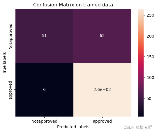
训练集和测试集上的混淆矩阵
# Get the confusion matrix for trained data

labels = ['Notapproved', 'approved']
cm = confusion_matrix(y_train, train_class_preds)
print(cm)

ax= plt.subplot()
sns.heatmap(cm, annot=True, ax = ax) #annot=True to annotate cells

# labels, title and ticks
ax.set_xlabel('Predicted labels')
ax.set_ylabel('True labels')
ax.set_title('Confusion Matrix on trained data')
ax.xaxis.set_ticklabels(labels)
ax.yaxis.set_ticklabels(labels)
plt.show()


# Get the confusion matrix for test data

labels = ['Notapproved', 'approved']
cm = confusion_matrix(y_test, test_class_preds)
print(cm)

ax= plt.subplot()
sns.heatmap(cm, annot=True, ax = ax); #annot=True to annotate cells

# labels, title and ticks
ax.set_xlabel('Predicted labels')
ax.set_ylabel('True labels')
ax.set_title('Confusion Matrix on test data')
ax.xaxis.set_ticklabels(labels)
ax.yaxis.set_ticklabels(labels)
[[ 51 62] [ 6 265]]
[[12 23]
 [ 0 61]]
[Text(0, 0.5, 'Notapproved'), Text(0, 1.5, 'approved')]

决策树
#Importing libraries
from sklearn.tree import DecisionTreeClassifier
from sklearn.model_selection import GridSearchCV
# applying GreadsearchCV to identify best parameters
decision_tree = DecisionTreeClassifier()
tree_para = {'criterion':['gini','entropy'],'max_depth':[4,5,6,7,8,9,10,11,12,15,20,30,40,50,70,90,120,150]}
clf = GridSearchCV(decision_tree, tree_para, cv=5)
clf.fit(X_train, y_train)
clf.best_params_{'criterion': 'gini', 'max_depth': 4}
#applying decision tree classifier
dt = DecisionTreeClassifier(criterion='gini',max_depth=4,random_state=0)
dt.fit(X_train, y_train)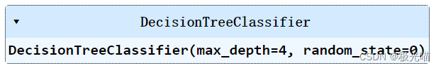
train_class_preds = dt.predict(X_train)
test_class_preds = dt.predict(X_test)
Accuracy Score
# Get the accuracy scores
train_accuracy = accuracy_score(train_class_preds,y_train)
test_accuracy = accuracy_score(test_class_preds,y_test)

print("The accuracy on train data is ", train_accuracy)
print("The accuracy on test data is ", test_accuracy)
The accuracy on train data is 0.8463541666666666 The accuracy on test data is 0.71875
roc_auc score
# Get the roc_auc scores
train_roc_auc = accuracy_score(y_train,train_class_preds)
test_roc_auc = accuracy_score(y_test,test_class_preds)

print("The accuracy on train data is ", train_roc_auc)
print("The accuracy on test data is ", test_roc_auc)
The accuracy on train data is 0.8463541666666666 The accuracy on test data is 0.71875
# Other evaluation metrics for train data
print(classification_report(train_class_preds,y_train))
precision recall f1-score support
0 0.54 0.90 0.67 68
1 0.97 0.84 0.90 316
accuracy 0.85 384
macro avg 0.76 0.87 0.79 384
weighted avg 0.90 0.85 0.86 384
# Other evaluation metrics for train data
print(classification_report(y_test,test_class_preds))
precision recall f1-score support
0 0.70 0.40 0.51 35
1 0.72 0.90 0.80 61
accuracy 0.72 96
macro avg 0.71 0.65 0.66 96
weighted avg 0.72 0.72 0.70 96
Confusion matrix on trained and test data
# Get the confusion matrix for trained data
labels = ['Notapproved', 'approved']
cm = confusion_matrix(y_train, train_class_preds)
print(cm)
ax= plt.subplot()
sns.heatmap(cm, annot=True, ax = ax) #annot=True to annotate cells
# labels, title and ticks
ax.set_xlabel('Predicted labels')
ax.set_ylabel('True labels')
ax.set_title('Confusion Matrix on trained data')
ax.xaxis.set_ticklabels(labels)
ax.yaxis.set_ticklabels(labels)
plt.show()
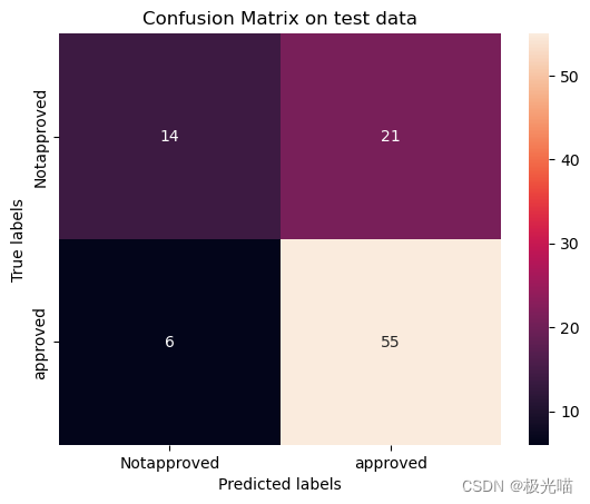
# Get the confusion matrix for test data
labels = ['Notapproved', 'approved']
cm = confusion_matrix(y_test, test_class_preds)
print(cm)
ax= plt.subplot()
sns.heatmap(cm, annot=True, ax = ax); #annot=True to annotate cells
# labels, title and ticks
ax.set_xlabel('Predicted labels')
ax.set_ylabel('True labels')
ax.set_title('Confusion Matrix on test data')
ax.xaxis.set_ticklabels(labels)
ax.yaxis.set_ticklabels(labels)[[ 61 52] [ 7 264]]

[[14 21]
 [ 6 55]]
[Text(0, 0.5, 'Notapproved'), Text(0, 1.5, 'approved')]
随机森林
# applying Random forrest classifier with Hyperparameter tuning
from sklearn.ensemble import RandomForestClassifier
rf = RandomForestClassifier()
grid_values = {'n_estimators':[50, 80,  100], 'max_depth':[4,5,6,7,8,9,10]}
rf_gd = GridSearchCV(rf, param_grid = grid_values, scoring = 'roc_auc', cv=5)

# Fit the object to train dataset
rf_gd.fit(X_train, y_train)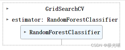
train_class_preds = rf_gd.predict(X_train)
test_class_preds = rf_gd.predict(X_test)
Accuracy Score
# Get the accuracy scores
train_accuracy = accuracy_score(train_class_preds,y_train)
test_accuracy = accuracy_score(test_class_preds,y_test)

print("The accuracy on train data is ", train_accuracy)
print("The accuracy on test data is ", test_accuracy)
The accuracy on train data is 0.890625 The accuracy on test data is 0.75
roc_auc Score
# Get the roc_auc scores
train_roc_auc = accuracy_score(y_train,train_class_preds)
test_roc_auc = accuracy_score(y_test,test_class_preds)

print("The accuracy on train data is ", train_roc_auc)
print("The accuracy on test data is ", test_roc_auc)
The accuracy on train data is 0.890625 The accuracy on test data is 0.75
Confusion Matrix
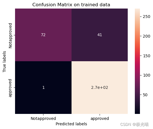
# Get the confusion matrix for trained data

labels = ['Notapproved', 'approved']
cm = confusion_matrix(y_train, train_class_preds)
print(cm)

ax= plt.subplot()
sns.heatmap(cm, annot=True, ax = ax) #annot=True to annotate cells

# labels, title and ticks
ax.set_xlabel('Predicted labels')
ax.set_ylabel('True labels')
ax.set_title('Confusion Matrix on trained data')
ax.xaxis.set_ticklabels(labels)
ax.yaxis.set_ticklabels(labels)
plt.show()

# Get the confusion matrix for test data

labels = ['Notapproved', 'approved']
cm = confusion_matrix(y_test, test_class_preds)
print(cm)

ax= plt.subplot()
sns.heatmap(cm, annot=True, ax = ax); #annot=True to annotate cells

# labels, title and ticks
ax.set_xlabel('Predicted labels')
ax.set_ylabel('True labels')
ax.set_title('Confusion Matrix on test data')
ax.xaxis.set_ticklabels(labels)
ax.yaxis.set_ticklabels(labels)
plt.show()
[[ 72 41] [ 1 270]]
[[13 22]
 [ 2 59]]
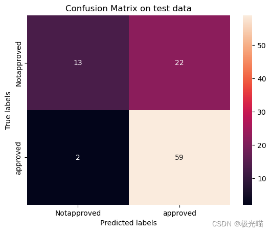
- 最佳 roc_auc 分数源于随机森林分类器,因此随机森林是该模型的最佳预测模型。