遥感影像纹理特征是描述影像中像素间空间关系的统计特征,常用于地物分类、目标识别和变化检测等遥感应用中。常见的纹理特征计算方式包括灰度共生矩阵(GLCM)、灰度差异矩阵(GLDM)、灰度不均匀性矩阵(GLRLM)等。这些方法通过对像素灰度值的统计分析,揭示了影像中像素间的空间分布规律,从而提取出纹理特征。
常用的纹理特征包括
1. 对比度(Contrast): 描述图像中灰度级之间的对比程度。
2. 同质性(Homogeneity): 描述图像中灰度级分布的均匀程度。
3. 熵(Entropy): 描述图像中灰度级分布的不确定性。
4. 方差(Variance): 描述图像中灰度级的离散程度。
5. 相关性(Correlation): 描述图像中像素间的灰度值相关程度。
6. 能量(Energy): 是灰度共生矩阵各元素值的平方和。
7. 均值(Mean): 描述图像中每个灰度级出现的平均频率。
8. 不相似度(Dissimilarity): 描述图像中不同灰度级之间的差异程度。
这些纹理特征可以通过GLCM等方法计算得到,用于描述遥感影像的纹理信息,对于遥感影像的分类和分析具有重要意义。
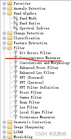
在ENVI中可以直接使用工具箱的工具直接计算得到输出影像
此外也可以使用python的skimage.feature库,这个库的greycoprops函数只有contrast、dissimilarity、homogeneity、ASM、energy和correlation这几个特征没有均值、方差和熵。因此下面对这个库的原函数进行修正,添加了方差等计算的greycoprops函数
def greycoprops(P, prop='contrast'):
    """Calculate texture properties of a GLCM.

    Compute a feature of a grey level co-occurrence matrix to serve as
    a compact summary of the matrix. The properties are computed as
    follows:

    - 'contrast': :math:`\\sum_{i,j=0}^{levels-1} P_{i,j}(i-j)^2`
    - 'dissimilarity': :math:`\\sum_{i,j=0}^{levels-1}P_{i,j}|i-j|`
    - 'homogeneity': :math:`\\sum_{i,j=0}^{levels-1}\\frac{P_{i,j}}{1+(i-j)^2}`
    - 'ASM': :math:`\\sum_{i,j=0}^{levels-1} P_{i,j}^2`
    - 'energy': :math:`\\sqrt{ASM}`
    - 'correlation':
        .. math:: \\sum_{i,j=0}^{levels-1} P_{i,j}\\left[\\frac{(i-\\mu_i) \\
                  (j-\\mu_j)}{\\sqrt{(\\sigma_i^2)(\\sigma_j^2)}}\\right]

    Each GLCM is normalized to have a sum of 1 before the computation of texture
    properties.

    Parameters
    ----------
    P : ndarray
        Input array. `P` is the grey-level co-occurrence histogram
        for which to compute the specified property. The value
        `P[i,j,d,theta]` is the number of times that grey-level j
        occurs at a distance d and at an angle theta from
        grey-level i.
    prop : {'contrast', 'dissimilarity', 'homogeneity', 'energy', \
            'correlation', 'ASM'}, optional
        The property of the GLCM to compute. The default is 'contrast'.

    Returns
    -------
    results : 2-D ndarray
        2-dimensional array. `results[d, a]` is the property 'prop' for
        the d'th distance and the a'th angle.

    References
    ----------
    .. [1] The GLCM Tutorial Home Page,
           http://www.fp.ucalgary.ca/mhallbey/tutorial.htm

    Examples
    --------
    Compute the contrast for GLCMs with distances [1, 2] and angles
    [0 degrees, 90 degrees]

    >>> image = np.array([[0, 0, 1, 1],
    ...                   [0, 0, 1, 1],
    ...                   [0, 2, 2, 2],
    ...                   [2, 2, 3, 3]], dtype=np.uint8)
    >>> g = greycomatrix(image, [1, 2], [0, np.pi/2], levels=4,
    ...                  normed=True, symmetric=True)
    >>> contrast = greycoprops(g, 'contrast')
    >>> contrast
    array([[0.58333333, 1.        ],
           [1.25      , 2.75      ]])

    """
    check_nD(P, 4, 'P')

    (num_level, num_level2, num_dist, num_angle) = P.shape
    if num_level != num_level2:
        raise ValueError('num_level and num_level2 must be equal.')
    if num_dist <= 0:
        raise ValueError('num_dist must be positive.')
    if num_angle <= 0:
        raise ValueError('num_angle must be positive.')

    # normalize each GLCM
    P = P.astype(np.float32)
    glcm_sums = np.apply_over_axes(np.sum, P, axes=(0, 1))
    glcm_sums[glcm_sums == 0] = 1
    P /= glcm_sums

    # create weights for specified property
    I, J = np.ogrid[0:num_level, 0:num_level]
    if prop == 'contrast':
        weights = (I - J) ** 2
    elif prop == 'dissimilarity':
        weights = np.abs(I - J)
    elif prop == 'homogeneity':
        weights = 1. / (1. + (I - J) ** 2)
    elif prop in ['ASM', 'energy', 'correlation', 'entropy', 'mean', 'variance']:
        pass
    else:
        raise ValueError('%s is an invalid property ?' % (prop))

    # compute property for each GLCM
    if prop == 'energy':
        asm = np.apply_over_axes(np.sum, (P ** 2), axes=(0, 1))[0, 0]
        results = np.sqrt(asm)
    elif prop == 'ASM':
        results = np.apply_over_axes(np.sum, (P ** 2), axes=(0, 1))[0, 0]
    elif prop == 'entropy':
        results = np.apply_over_axes(np.sum, -P * np.log10(P+0.00001), axes=(0, 1))[0, 0]
    elif prop == 'correlation':
        results = np.zeros((num_dist, num_angle), dtype=np.float64)
        I = np.array(range(num_level)).reshape((num_level, 1, 1, 1))
        J = np.array(range(num_level)).reshape((1, num_level, 1, 1))
        diff_i = I - np.apply_over_axes(np.sum, (I * P), axes=(0, 1))[0, 0]
        diff_j = J - np.apply_over_axes(np.sum, (J * P), axes=(0, 1))[0, 0]

        std_i = np.sqrt(np.apply_over_axes(np.sum, (P * (diff_i) ** 2),
                                           axes=(0, 1))[0, 0])
        std_j = np.sqrt(np.apply_over_axes(np.sum, (P * (diff_j) ** 2),
                                           axes=(0, 1))[0, 0])
        cov = np.apply_over_axes(np.sum, (P * (diff_i * diff_j)),
                                 axes=(0, 1))[0, 0]

        # handle the special case of standard deviations near zero
        mask_0 = std_i < 1e-15
        mask_0[std_j < 1e-15] = True
        results[mask_0] = 1

        # handle the standard case
        mask_1 = mask_0 == False
        results[mask_1] = cov[mask_1] / (std_i[mask_1] * std_j[mask_1])
    elif prop in ['contrast', 'dissimilarity', 'homogeneity']:
        weights = weights.reshape((num_level, num_level, 1, 1))
        results = np.apply_over_axes(np.sum, (P * weights), axes=(0, 1))[0, 0]
    elif prop == 'mean':
        I = np.array(range(num_level)).reshape((num_level, 1, 1, 1))
        results = np.apply_over_axes(np.sum, (P * I), axes=(0, 1))[0, 0]
    elif prop == 'variance':
        I = np.array(range(num_level)).reshape((num_level, 1, 1, 1))
        mean = np.apply_over_axes(np.sum, (P * I), axes=(0, 1))[0, 0]
        results = np.apply_over_axes(np.sum, (P * (I - mean) ** 2), axes=(0, 1))[0, 0]

    return results
具体影像分析时还需要考虑灰色关联矩阵计算的角度、步长、灰度级数和窗口大小。以一张多光谱影像为例,相关性使用了greycoprops,其他的特征使用公式计算,实际上导入上面的新greycoprops函数后其他特征都可以用函数计算,具体代码如下,输出结果为多光谱各个波段的纹理特征的多通道影像:
from osgeo import gdal, osr
import os
import numpy as np
import cv2
from skimage import data
from skimage.feature import greycoprops

def export_tif(out_tif_name, var_lat, var_lon, NDVI, bandname=None):
    # 判断数组维度
    if len(NDVI.shape) > 2:
        im_bands, im_height, im_width = NDVI.shape
    else:
        im_bands, (im_height, im_width) = 1, NDVI.shape
    LonMin, LatMax, LonMax, LatMin = [min(var_lon), max(var_lat), max(var_lon), min(var_lat)]
    # 分辨率计算
    Lon_Res = (LonMax - LonMin) / (float(im_width) - 1)
    Lat_Res = (LatMax - LatMin) / (float(im_height) - 1)
    driver = gdal.GetDriverByName('GTiff')
    out_tif = driver.Create(out_tif_name, im_width, im_height, im_bands, gdal.GDT_Float32)  # 创建框架

    # 设置影像的显示范围
    # Lat_Res一定要是-的
    geotransform = (LonMin, Lon_Res, 0, LatMax, 0, -Lat_Res)
    out_tif.SetGeoTransform(geotransform)

    # 获取地理坐标系统信息,用于选取需要的地理坐标系统
    srs = osr.SpatialReference()
    srs.ImportFromEPSG(4326)  # 定义输出的坐标系为"WGS 84",AUTHORITY["EPSG","4326"]
    out_tif.SetProjection(srs.ExportToWkt())  # 给新建图层赋予投影信息

    # 数据写出
    if im_bands == 1:
        out_tif.GetRasterBand(1).WriteArray(NDVI)
    else:
        for bands in range(im_bands):
            # 为每个波段设置名称
            if bandname is not None:
                out_tif.GetRasterBand(bands + 1).SetDescription(bandname[bands])
            out_tif.GetRasterBand(bands + 1).WriteArray(NDVI[bands])

    # 生成 ENVI HDR 文件
    hdr_file = out_tif_name.replace('.tif', '.hdr')
    with open(hdr_file, 'w') as f:
        f.write('ENVI\n')
        f.write('description = {Generated by export_tif}\n')
        f.write('samples = {}\n'.format(im_width))
        f.write('lines   = {}\n'.format(im_height))
        f.write('bands   = {}\n'.format(im_bands))
        f.write('header offset = 0\n')
        f.write('file type = ENVI Standard\n')
        f.write('data type = {}\n'.format(gdal.GetDataTypeName(out_tif.GetRasterBand(1).DataType)))
        f.write('interleave = bsq\n')
        f.write('sensor type = Unknown\n')
        f.write('byte order = 0\n')
        band_names_str = ', '.join(str(band) for band in bandname)
        f.write('band names = {%s}\n'%(band_names_str))

    del out_tif


def fast_glcm(img, vmin=0, vmax=255, levels=8, kernel_size=5, distance=1.0, angle=0.0):
    '''
    Parameters
    ----------
    img: array_like, shape=(h,w), dtype=np.uint8
        input image
    vmin: int
        minimum value of input image
    vmax: int
        maximum value of input image
    levels: int
        number of grey-levels of GLCM
    kernel_size: int
        Patch size to calculate GLCM around the target pixel
    distance: float
        pixel pair distance offsets [pixel] (1.0, 2.0, and etc.)
    angle: float
        pixel pair angles [degree] (0.0, 30.0, 45.0, 90.0, and etc.)

    Returns
    -------
    Grey-level co-occurrence matrix for each pixels
    shape = (levels, levels, h, w)
    '''

    mi, ma = vmin, vmax
    ks = kernel_size
    h,w = img.shape

    # digitize
    bins = np.linspace(mi, ma+1, levels+1)
    gl1 = np.digitize(img, bins) - 1

    # make shifted image
    dx = distance*np.cos(np.deg2rad(angle))
    dy = distance*np.sin(np.deg2rad(-angle))
    mat = np.array([[1.0,0.0,-dx], [0.0,1.0,-dy]], dtype=np.float32)
    gl2 = cv2.warpAffine(gl1, mat, (w,h), flags=cv2.INTER_NEAREST,
                         borderMode=cv2.BORDER_REPLICATE)

    # make glcm
    glcm = np.zeros((levels, levels, h, w), dtype=np.uint8)
    for i in range(levels):
        for j in range(levels):
            mask = ((gl1==i) & (gl2==j))
            glcm[i,j, mask] = 1

    kernel = np.ones((ks, ks), dtype=np.uint8)
    for i in range(levels):
        for j in range(levels):
            glcm[i,j] = cv2.filter2D(glcm[i,j], -1, kernel)
    # 灰色关联矩阵归一化,之后结果与ENVI相同
    glcm = glcm.astype(np.float32)
    glcm_sums = np.apply_over_axes(np.sum, glcm, axes=(0, 1))
    glcm_sums[glcm_sums == 0] = 1
    glcm /= glcm_sums
    return glcm


def fast_glcm_texture(img, vmin=0, vmax=255, levels=8, ks=5, distance=1.0, angle=0.0):
    '''
    calc glcm texture
    '''
    h,w = img.shape
    glcm = fast_glcm(img, vmin, vmax, levels, ks, distance, angle)
    mean = np.zeros((h,w), dtype=np.float32)
    var = np.zeros((h,w), dtype=np.float32)
    cont = np.zeros((h,w), dtype=np.float32)
    diss = np.zeros((h,w), dtype=np.float32)
    homo = np.zeros((h,w), dtype=np.float32)
    asm = np.zeros((h,w), dtype=np.float32)
    ent = np.zeros((h,w), dtype=np.float32)
    cor = np.zeros((h, w), dtype=np.float32)

    for i in range(levels):
        for j in range(levels):
            mean += glcm[i,j] * i
            homo += glcm[i,j] / (1.+(i-j)**2)
            asm  += glcm[i,j]**2
            cont += glcm[i,j] * (i-j)**2
            diss += glcm[i,j] * np.abs(i-j)
            ent -= glcm[i, j] * np.log10(glcm[i, j] + 0.00001)
    for i in range(levels):
        for j in range(levels):
            var += glcm[i, j] * (i - mean)**2
    greycoprops(glcm, 'correlation')  # 上面计算的几个特征均可这样写
    cor[cor == 1.0] = 0.
    homo[homo == 1.] = 0
    asm[asm == 1.] = 0
    return [mean, var, cont, diss, homo, asm, ent, cor]

# 遥感影像
image = r'..\path\to\your\file\image.tif'
# 文件输出路径
out_path = r'..\output\path'
dataset = gdal.Open(image)  # 读取数据
adfGeoTransform = dataset.GetGeoTransform()
nXSize = dataset.RasterXSize  # 列数
nYSize = dataset.RasterYSize  # 行数
im_data = dataset.ReadAsArray(0, 0, nXSize, nYSize)  # 读取数据
im_data[im_data==65536] = 0
var_lat = []  # 纬度
var_lon = []  # 经度
for j in range(nYSize):
    lat = adfGeoTransform[3] + j * adfGeoTransform[5]
    var_lat.append(lat)
for i in range(nXSize):
    lon = adfGeoTransform[0] + i * adfGeoTransform[1]
    var_lon.append(lon)
result = []
band_name=[]
for i, img in enumerate(im_data):
    img = np.uint8(255.0 * (img - np.min(img))/(np.max(img) - np.min(img))) # normalization
    fast_result = fast_glcm_texture(img, vmin=0, vmax=255, levels=32, ks=3, distance=1.0, angle=0.0)
    result += fast_result
    variable_names = ['mean', 'variance', 'contrast', 'dissimilarity', 'homogeneity', 'ASM', 'entropy', 'correlation']
    for names in variable_names:
        band_name.append('band_'+str(i+1)+'_'+names)
name = os.path.splitext(os.path.basename(image))[0]
export_tif(os.path.join(out_path, '%s_TF.tif' % name), var_lat, var_lon, np.array(result), bandname=band_name)
print('over')
总结
目前熵值特征计算结果与ENVI有差异,不过只是数值差异,使用影像打开的结果显示一致,说明只是值的范围差异,不影响分析,其他特征均与ENVI的计算结果一致