pytorch——房价预测

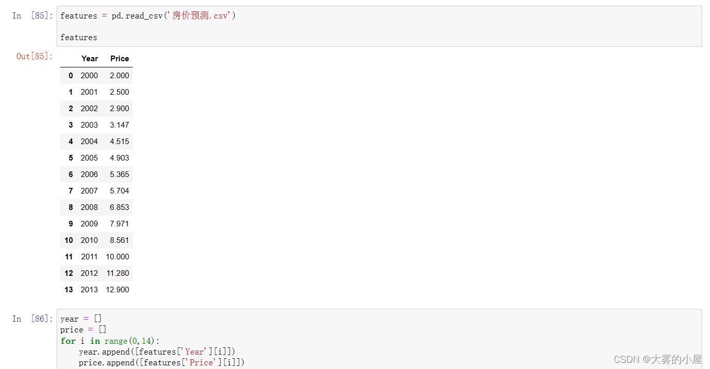
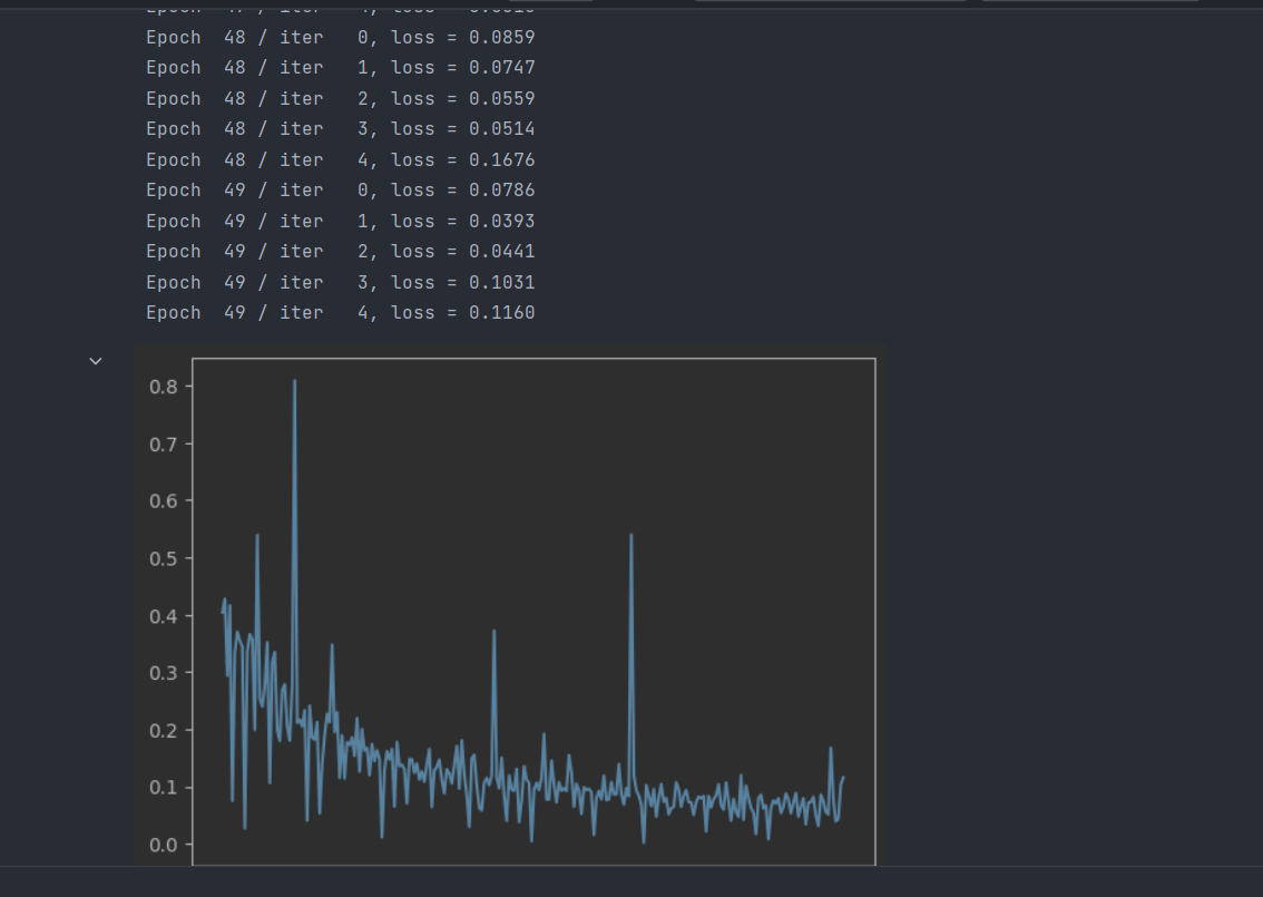
1、首先对数据进行读取和预处理 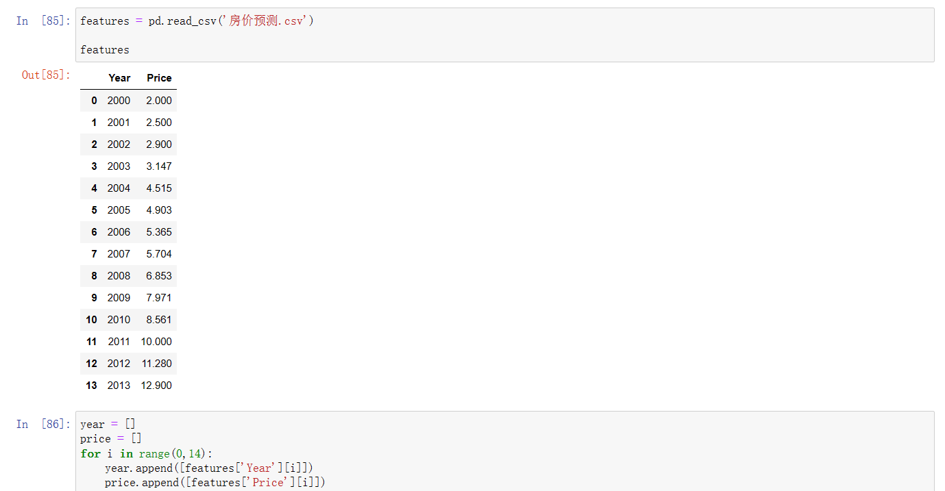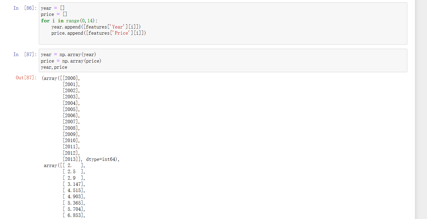2、读取数据后，对x数据进行标准化处理，以便于后续训练的稳定性，并转换为tensor格式 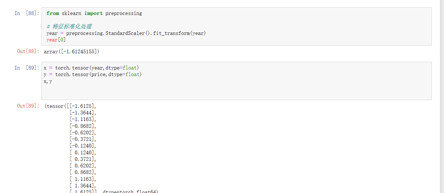3、接下来设置训练参数和模型 这里采用回归模型，既y=x*weight1+bias1，设置的学习率为0.0006，损失函数采用了MSE（均方误差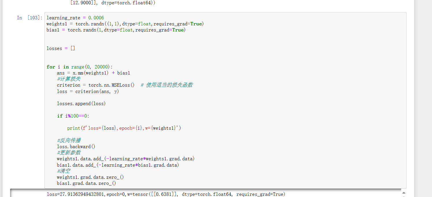） 4、绘制图像 由于数据量较少，所以将整个训练集作为测试集，观察生成的图像

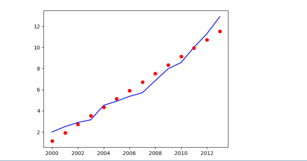
完整代码

import torch
import numpy as np
import pandas as pd
import matplotlib.pyplot as plt
import torch.optim as optim
import warnings
warnings.filterwarnings("ignore")


# In[4]:


features = pd.read_csv('房价预测.csv')

features


# In[26]:


year = []
price = []
for i in range(0,12):
    year.append([features['Year'][i]])
    price.append([features['Price'][i]])



# In[27]:


year = np.array(year)
price = np.array(price)
year,price


# In[53]:


from sklearn import preprocessing

# 特征标准化处理
year = preprocessing.StandardScaler().fit_transform(year)
year[0]


# In[54]:


x = torch.tensor(year,dtype=float)
y = torch.tensor(price,dtype=float)
x,y


# In[62]:


learning_rate = 0.0001
weights1 = torch.randn((1,1),dtype=float,requires_grad=True)
bias1 = torch.randn(1,dtype=float,requires_grad=True)


losses = []


for i in range(0, 5000):
    ans = x.mm(weights1) + bias1
    #计算损失
    criterion = torch.nn.MSELoss()  # 使用适当的损失函数
    loss = criterion(ans, y)

    losses.append(loss)

    if i%100==0:

        print(f'loss={loss},epoch={i},w={weights1}')

    #反向传播
    loss.backward()
    #更新参数
    weights1.data.add_(-learning_rate*weights1.grad.data)
    bias1.data.add_(-learning_rate*bias1.grad.data)
    #清空
    weights1.grad.data.zero_()
    bias1.grad.data.zero_()
# 使用 features['Year'] 和 features['Price'] 创建日期和价格的列表
year = features['Year']
price = features['Price']
# 将 ans 转换为 Python 列表
ans_list = ans.tolist()

# 提取列表中的每个元素（确保是单个的标量值）
predictions = [item[0] for item in ans_list]

# 创建一个表格来存日期和其对应的标签数值
true_data = pd.DataFrame(data={'date': year, 'actual': price})
predictions_data = pd.DataFrame(data={'date': year, 'prediction': predictions})
# 真实值
plt.plot(true_data['date'], true_data['actual'], 'b-', label='actual')

# 预测值
plt.plot(predictions_data['date'], predictions_data['prediction'], 'ro', label='prediction')
plt.xticks(rotation='60')
plt.legend()

# 图名
plt.xlabel('Date')
plt.ylabel('Price')  # 注意修改为你的标签
plt.title('Actual and Predicted Values')
plt.show()

本文由博客一文多发平台 OpenWrite 发布！