逻辑回归 使用Numpy实现逻辑回归

使用Numpy实现逻辑回归

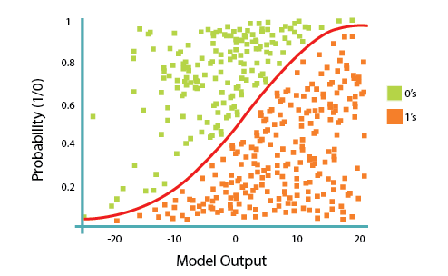
sigmoid 函数

$g(z)=\frac{1}{(1+e^{-z})}$

# sigmoid 函数
def sigmod(z):
    return 1/(1+np.exp(-z))

线性计算与梯度下降

$$J(\theta )=-\frac{1}{m}[\sum _{i=1}^m{y}^{(i)}log(h_{\theta }(x^{(i)}))+(1-y^{(i)})log(1-h_{\theta }(x^{(i)}))]$$

对于代价函数，采用梯度下降算法求θ的最小值：
$${\theta }_j:={\theta }_j-\alpha \frac{\partial J(\theta )}{\partial {\theta }_j}$$
代入梯度：
$${\theta }_j:={\theta }_j-\alpha \sum _{i=1}^m(h_{\theta }(x^{(i)})-y^{(i)})x_j^i$$

# 进行计算
def compute(X,y,weights,bias):
    count=len(X)
    linear=np.dot(X,weights)+bias
    
    predictions = sigmoid(linear)
    
    dw=(1/count)*np.dot(X.T,(predictions-y))
    db=(1/count)*np.sum(predictions-y)
    
    return dw,db

def update(weights,bias,dw,db,rate):
    weights=weights-rate*dw
    bias=bias-rate*db
    
    return weights,bias

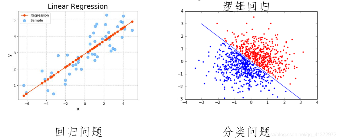
实现逻辑回归

逻辑回归公式
$$h_{\theta }(x)=\frac{1}{(1+e^{-{\theta }^{T}X})}$$

#逻辑回归
def logistic(X,y,rate,iterations):
    count,col=X.shape
    weights,bias=initialize(col)
    
    for _ in range(iterations):
        dw,db=compute(X,y,weights,bias)
        
        weights,bias =update(weights,bias,dw,db,rate)
        
    return weights, bias

测试模型

import numpy as np
import matplotlib.pyplot as plt

# 生成两个特征的单调数据
np.random.seed(42)
X1 = np.linspace(1, 5, 100) + np.random.randn(100) * 0.2
X2 = np.linspace(1, 5, 100) + np.random.randn(100) * 0.2
X = np.column_stack((X1, X2))

# 生成对应的标签，假设以直线 x1 = x2 为界限进行二分类
y = (X[:, 0] > X[:, 1]).astype(int)

# 添加偏置项
X_with_bias = np.c_[np.ones((X.shape[0], 1)), X]

# 训练逻辑回归模型
weights, bias = logistic(X_with_bias, y, rate=0.1, iterations=1000)

# 选择一些数据点进行预测
X_predict = np.array([[2, 2], [3, 4], [4, 3]])
predictions = predict(np.c_[np.ones((X_predict.shape[0], 1)), X_predict], weights, bias)

# 输出预测结果
print("Predictions:", predictions)

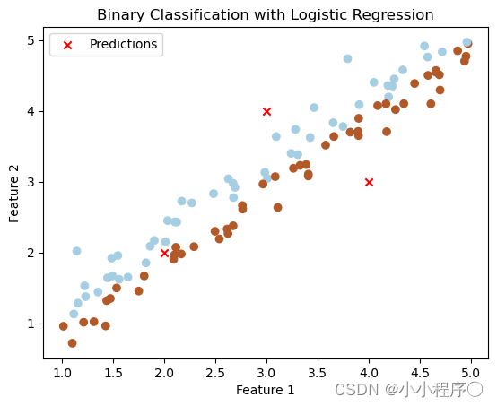
# 画出二分类后的图
plt.scatter(X[:, 0], X[:, 1], c=y, cmap=plt.cm.Paired, marker='o')
plt.scatter(X_predict[:, 0], X_predict[:, 1], marker='x', color='red', label='Predictions')
plt.xlabel('Feature 1')
plt.ylabel('Feature 2')
plt.title('Binary Classification with Logistic Regression')
plt.legend()
plt.show()

完整代码

import numpy as np

# sigmoid 函数
def sigmod(z):
    return 1/(1+np.exp(-z))

# 初始化参数
def initialize(num_col):
    weights=np.zeros(num_col)
    bias=0
    return weights,bias

# 进行计算
def compute(X,y,weights,bias):
    count=len(X)
    linear=np.dot(X,weights)+bias
    
    predictions = sigmoid(linear)
    
    dw=(1/count)*np.dot(X.T,(predictions-y))
    db=(1/count)*np.sum(predictions-y)
    
    return dw,db

# 梯度下降
def update(weights,bias,dw,db,rate):
    weights=weights-rate*dw
    bias=bias-rate*db
    
    return weights,bias
    
#逻辑回归
def logistic(X,y,rate,iterations):
    count,col=X.shape
    weights,bias=initialize(col)
    
    for _ in range(iterations):
        dw,db=compute(X,y,weights,bias)
        
        weights,bias =update(weights,bias,dw,db,rate)
        
    return weights, bias

# 预测结果
def predict(X,weights,bias):
    linear = np.dot(X,weights)+bias
    predictions=sigmoid(linear)
    
    return [1 if y_hat>0.5 else 0  for y_hat in predictions]

可视化代码

import numpy as np
import matplotlib.pyplot as plt

# 生成两个特征的单调数据
np.random.seed(42)
X1 = np.linspace(1, 5, 100) + np.random.randn(100) * 0.2
X2 = np.linspace(1, 5, 100) + np.random.randn(100) * 0.2
X = np.column_stack((X1, X2))

# 生成对应的标签，假设以直线 x1 = x2 为界限进行二分类
y = (X[:, 0] > X[:, 1]).astype(int)

# 添加偏置项
X_with_bias = np.c_[np.ones((X.shape[0], 1)), X]

# 训练逻辑回归模型
weights, bias = logistic(X_with_bias, y, rate=0.1, iterations=1000)

# 选择一些数据点进行预测
X_predict = np.array([[2, 2], [3, 4], [4, 3]])
predictions = predict(np.c_[np.ones((X_predict.shape[0], 1)), X_predict], weights, bias)

# 输出预测结果
print("Predictions:", predictions)

# 画出二分类后的图
plt.scatter(X[:, 0], X[:, 1], c=y, cmap=plt.cm.Paired, marker='o')
plt.scatter(X_predict[:, 0], X_predict[:, 1], marker='x', color='red', label='Predictions')
plt.xlabel('Feature 1')
plt.ylabel('Feature 2')
plt.title('Binary Classification with Logistic Regression')
plt.legend()
plt.show()