Consider the fractional knapsack problem defined as follows. Given n items of sizes s1, s2, . . . , sn, and values v1, v2, . . . , vn and size C, the knapsack capacity, the objective is to find nonnegative real numbers x1, x2, . . . , xn, 0 ≤ xi ≤ 1, that maximize the sum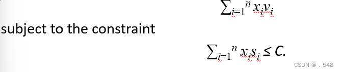
n=3, M=20,
(s1,s2,s3)=(18,15,10), (v1,v2,v3)=(25,24,15).
(As We can be seen from the example, this greedy criterion is not optimal)
(As We can be seen from the example, this greedy criterion is not optimal)
The Shortest Path Problem
Let G = (V,E) be a directed graph in which each edge has a nonnegative length, and there is a distinguished vertex s called the source. The single source shortest path problem, or simply the shortest path problem, is to determine the distance from s to every other vertex in V , where the distance from vertex s to vertex x is defined as the length of a shortest path from s to x.
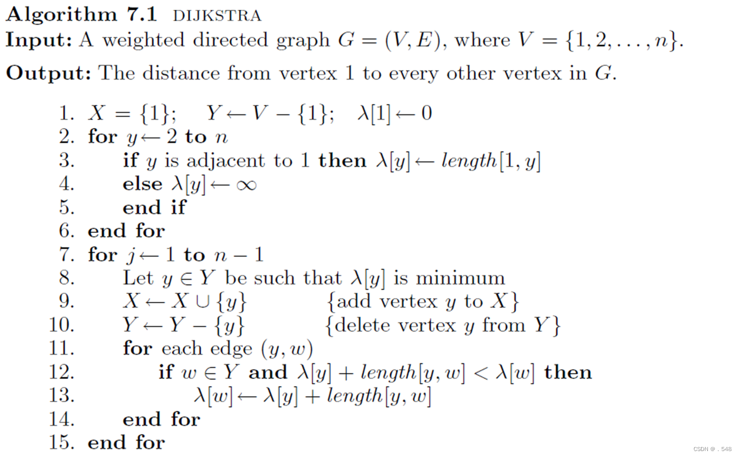
(1) X ←{1}; Y ←V −{1}
(2) For each vertex v ∈ Y if there is an edge from 1 to v then let λ[v] (the label of v) be the length of that edge; otherwise let λ[v] = ∞.Let λ[1] = 0.
(3) while Y = {}
(4) Let y ∈ Y be such that λ[y] is minimum.
(5) move y from Y to X.
(6) update the labels of those vertices in Y that are adjacent to y.
(7) end while
Example 7.2 To see how the algorithm works, consider the directed graph shown in Fig. 7.1(a). The first step is to label each vertex v with λ[v] = length[1, v]. As shown in the figure, vertex 1 is labeled with 0, and vertices 2 and 3 are labeled with 1 and 12, respectively since length[1, 2] = 1 and length[1, 3] = 12. All other vertices are labeled with ∞ since there are no edges from the source vertex to these vertices. Initially X = {1} and Y = {2, 3, 4, 5, 6}. In the figure, those vertices to the left of the dashed line belong to X, and the others belong to Y .
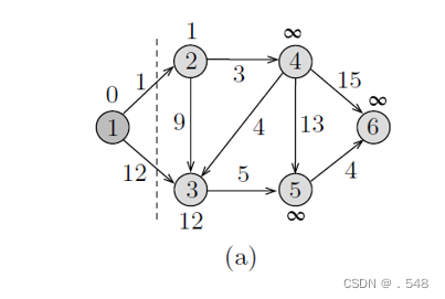
In Fig. 7.1(a), we note that λ[2] is the smallest among all vertices’ labels in Y , and hence it is moved to X, indicating that the distance to vertex 2 has been found. To finish processing vertex 2, the labels of its neighbors 3 and 4 are inspected to see if there are paths that pass through 2 and are shorter than their old paths. In this case, we say that we update the labels of the vertices adjacent to 2. As shown in the figure, the path from 1 to 2 to 3 is shorter than the path from 1 to 3, and thus λ[3] is changed to 10, which is the length of the path that passes through 2. Similarly, λ[4] is changed to 4 since now there is a finite path of length 4 from 1 to 4 that passes through vertex 2. These updates are shown in Fig. 7.1(b).
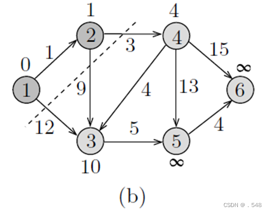
The next step is to move that vertex with minimum label, namely 4, to X and update the labels of its neighbors in Y as shown in Fig. 7.1(c). In this figure, we notice that the labels of vertices 5 and 6 became finite and λ[3] is lowered to 8. Now, vertex 3 has a minimum label, so it is moved to X and λ[5] is updated accordingly as shown in Fig. 7.1(d).

Continuing in this way, the distance to vertex 5 is found and thus it is moved to X as shown in Fig. 7.1(e). As shown in Fig. 7.1(f), vertex 6 is the only vertex remaining in Y and hence its label coincides with the length of its distance from 1. In Fig. 7.1(f), the label of each vertex represents its distance from the source vertex.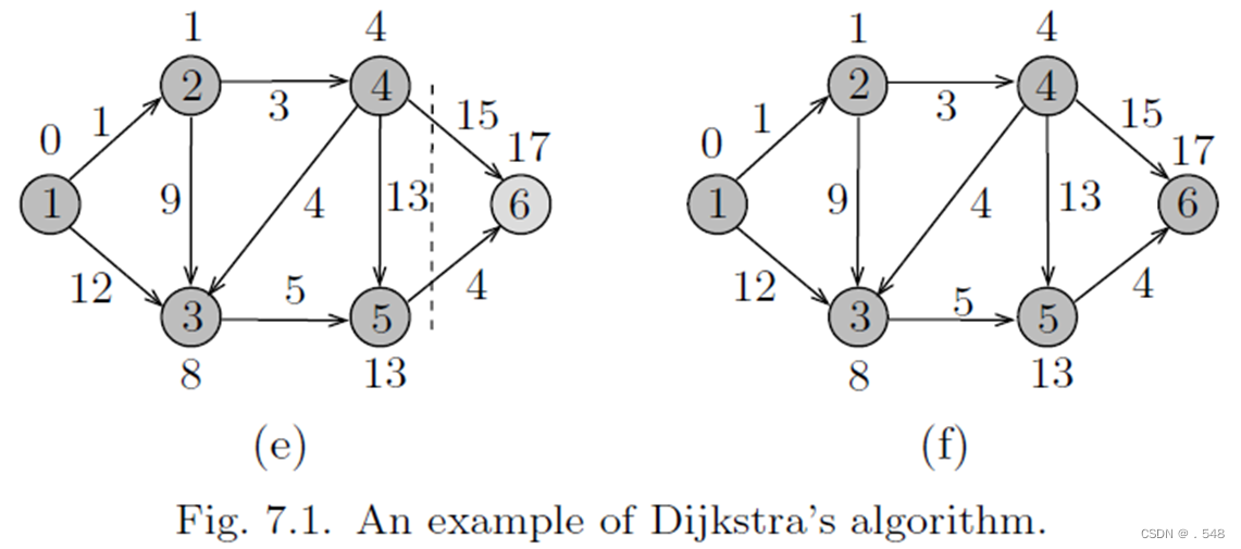
Lemma 7.1 In Algorithm DIJKSTRA, when a vertex y is chosen in Step 8, if λ[y] ]<∞, then λ[y] = δ[y].
λ[y] ≤ λ[w] sincey left Y before w
≤ λ[x] + length(x,w) by the algorithm
= δ[x] + length(x,w) by induction
= δ[w] sinceπ is a path of shortest length
≤ δ[y] sinceπ is a path of shortest length.
Theorem 7.1 Given a directed graph G with nonnegative weights on its edges and a source vertex s, Algorithm DIJKSTRA finds the length of the distance from s to every other vertex in Θ(n2) time.
Minimum Cost Spanning Trees
Let G = (V,E) be a connected undirected graph with weights on its edges. A spanning tree (V, T) of G is a subgraph of G that is a tree. If G is weighted and the sum of the weights of the edges in T is minimum, then (V, T) is called a minimum cost spanning tree or simply a minimum spanning tree.
Given an undirected weighted graph G=<V, E>, it is required to find a minimum spanning tree of G.
The algorithm requires selecting n-1 edges. Its greedy criterion: select the edge with the smallest weight from the remaining edges, and its addition should still form a tree with the already selected edge set.
The algorithm requires selecting n-1 edges. Its greedy criterion: select an edge with the minimum weight from the remaining edges that does not form a cricle (i.e. a loop) with the already selected edge set
The algorithm gets the minimum spanning tree by deleting several edges from the original graph. Its greedy criterion: Select any circuit in the remaining graph and remove one of its maximum weight edges to break the circuit.
Minimum Cost Spanning Trees
(Kruskal’s Algorithm)
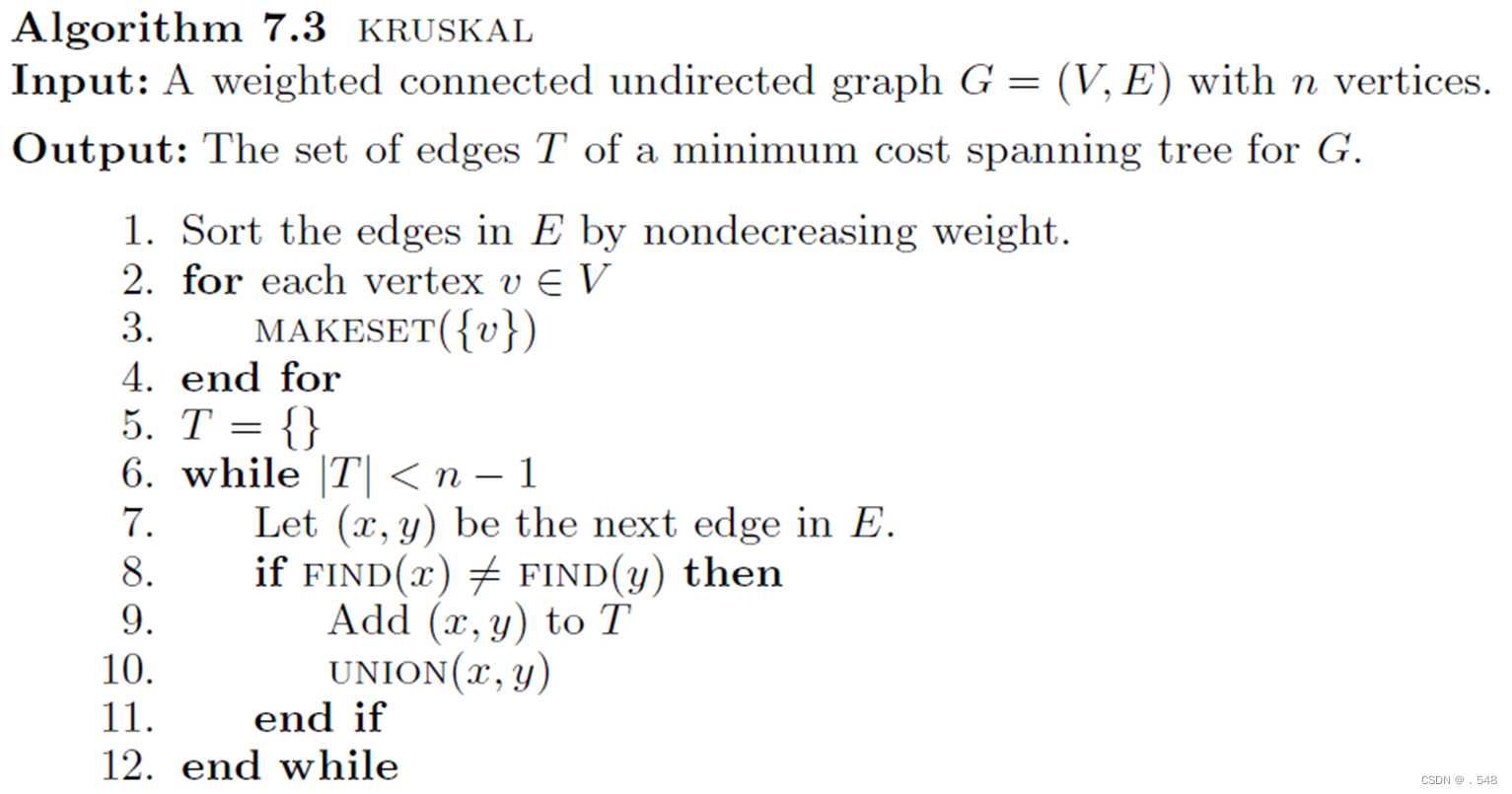
(1) Sort the edges in G by nondecreasing weight, let T={}.
(2) For each edge in the sorted list, include that edge in the spanning tree T if it does not form a cycle with the edges currently included in T; otherwise, discard it.
Example 7.3 Consider the weighted graph shown in Fig. 7.4(a). As shown in Fig. 7.4(b), the first edge that is added is (1, 2) since it is of minimum cost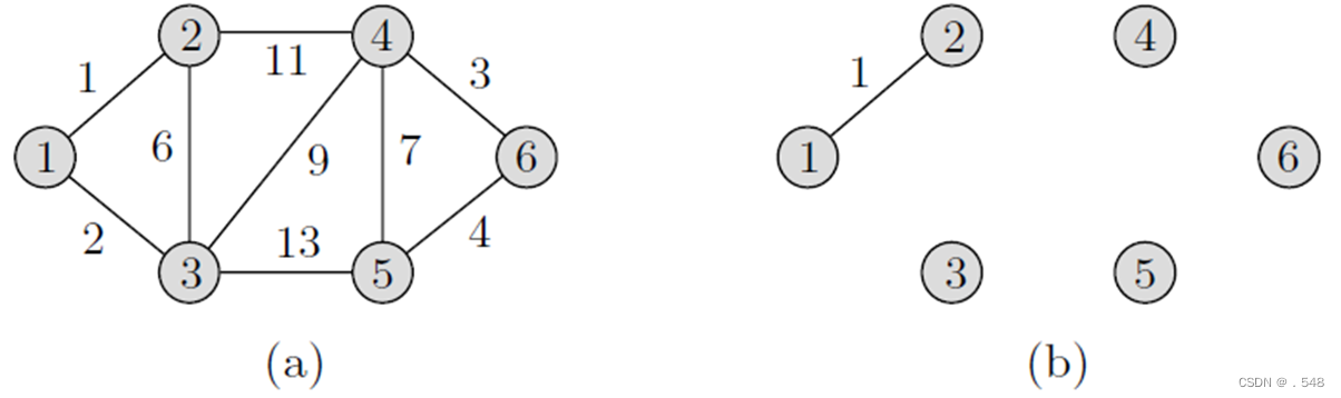
Next, as shown in Fig. 7.4(c)–(e), edges (1, 3), (4, 6), and then (5, 6) are included in T in this order.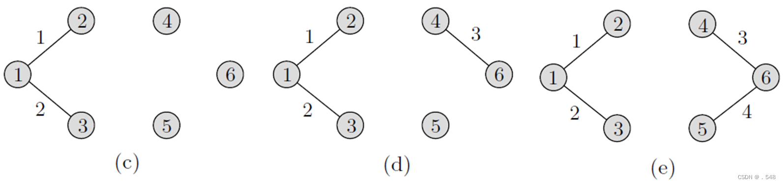 Next, as shown in Fig. 7.4(f), the edge (2, 3) creates a cycle and hence is discarded. For the same reason, as shown in Fig. 7.4(g), edge (4, 5) is also discarded. Finally, edge (3, 4) is included, which results in the minimum spanning tree (V, T) shown in Fig. 7.4(h).
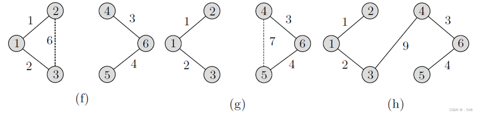
Suppose we are given a set S of n distinct elements. The elements are partitioned into disjoint sets. There are union and find operations on S.
In each subset, a distinguished element will serve as the name of the set or set representative. For example, if S = {1, 2, . . . , 11} and there are 4 subsets {1, 7, 10, 11}, {2, 3, 5, 6}, {4, 8}, and {9}, these subsets may be labeled as 1, 3, 8, and 9, in this order. The find operation returns the name of the set containing a particular element. For example, executing the operation find(11) returns 1, the name of the set containing 11. These two operations are defined more precisely as follows:
The goal is to design efficient algorithms for these two operations. To achieve this, we need a data structure that is both simple and at the same time allows for the efficient implementation of the union and find operations
The disjoint sets can be represented
by two ways:
(a) Tree representation.
(b) Array representation when
S = {1, 2, . . . , n}.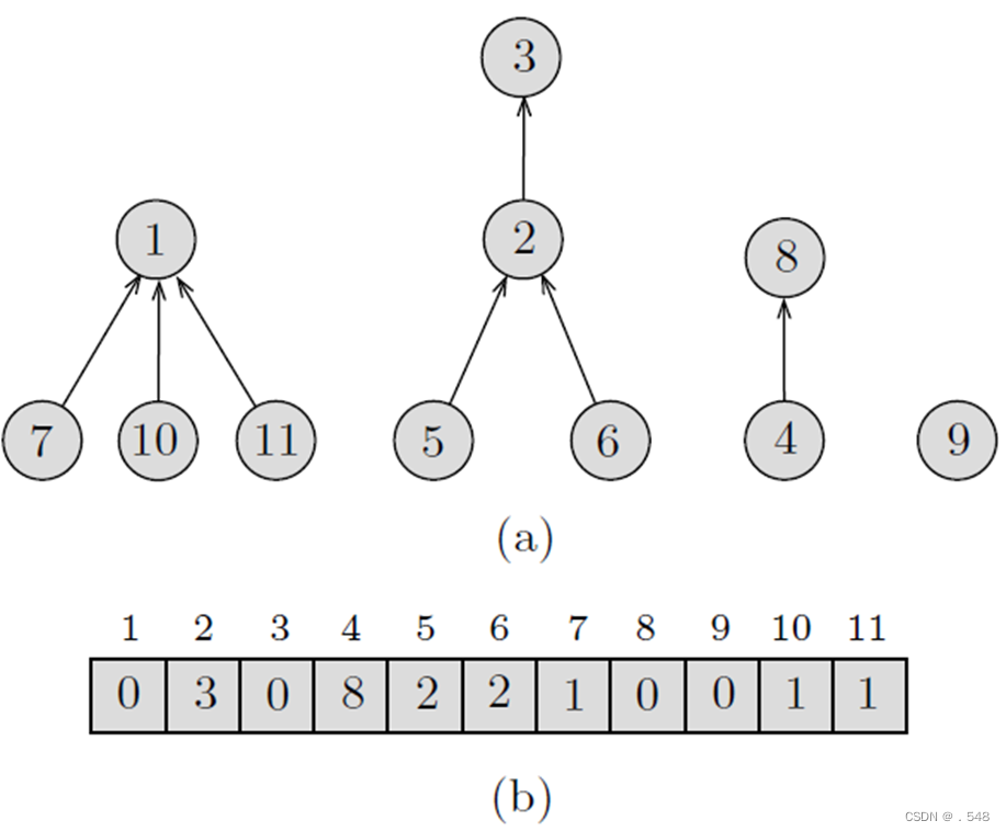
(a) Tree representation
Each element x other than the root has a pointer to its parent p(x) in the tree. The root has a null pointer, and it serves as the name or set representative of the set. This results in a forest in which each tree corresponds to one set.
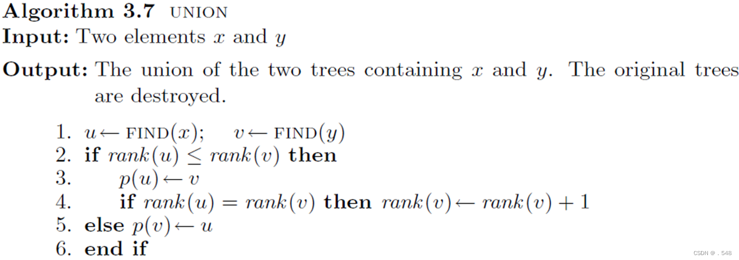
For any element x, let root(x) denote the root of the tree containing x. Thus, find(x) always returns root(x). As the union operation must have as its arguments the roots of two trees, we will assume that for any two elements x and y, union(x, y) actually means union(root(x), root(y)).
(b) Array representation
If we assume that the elements are the integers 1, 2, . . . , n, the forest can conveniently be represented by an array A[1..n] such that A[j] is the parent of element j, 1 ≤ j ≤ n. The null parent can be represented by the number 0.
Clearly, since the elements are consecutive integers, the array representation is preferable. However, in developing the algorithms for the union and find operations, we will assume the more general representation, that is, the tree representation.
Suppose we start with the singletonsets {1}, {2}, . . . , {n} and
then execute the following sequence of unions and finds
(see Fig(a)):
union(1, 2), union(2, 3), . . . , union(n − 1, n),
find(1), find(2), . . . , find(n).
In this case, the total cost of the n find operations is
proportional to
n + (n − 1) + ・ ・ ・+ 1 = n(n + 1)/2= Θ(n2).
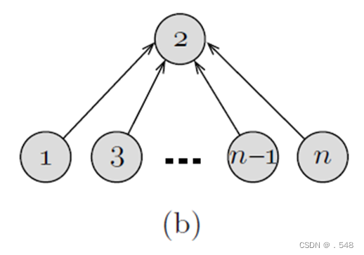
In order to constraint the height of each tree, we adopt the union by rank heuristic: We store with each node a nonnegative number referred to as the rank of that node. The rank of a node is essentially its height. Let x and y be two roots of two different trees in the current forest. Initially, each node has rank 0. When performing the operation union(x, y), we compare rank (x) and rank (y). If rank (x) < rank (y), we make y the parent of x. If rank (x) > rank (y), we make x the parent of y. Otherwise, if rank (x) = rank (y), we make y the parent of x and increase rank (y) by 1. Applying this rule on the sequence of operations above yields the tree shown in Fig. 3.6(b). Note that the total cost of the n find operations is now reduced to Θ(n). This, however, is not always the case. As will be shown later, using this rule, the time required to process n finds is O(n log n).
Observation 3.1 rank (p(x)) ≥ rank (x) + 1.
Observation 3.2 The value of rank (x) is initially zero and increases in subsequent union operations until x is no longer a root. Once x becomes a child of another node, its rank never changes.Lemma 3.1 The number of nodes in a tree with root x is at least 2**rank(x).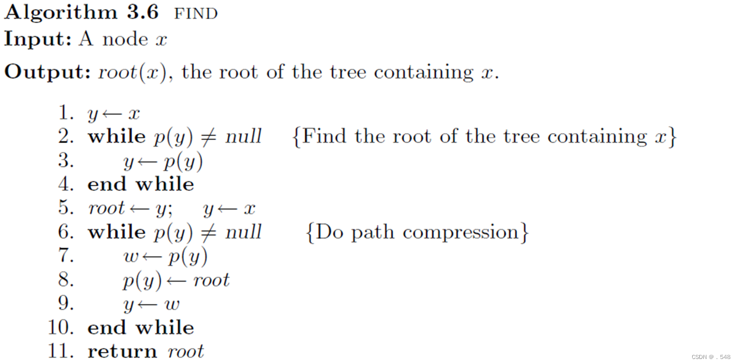
 Example 3.4 Let S = {1, 2, . . . , 9} and consider applying the following sequence of unions and finds: union(1, 2), union(3, 4), union(5, 6), union(7, 8), union(2, 4), union(8, 9), union(6, 8), find(5), union(4, 8), find(1). Figure 3.8(a) shows the initial configuration. Figure 3.8(b) shows the data structure after the first four union operations. The result of the next three union operations is shown in Fig. 3.8(c). Figure 3.8(d) shows the effect of executing the operation find(5). The results of the operations union(4, 8) and find(1) are shown in Fig. 3.8(e) and (f), respectively.
  Time complexity: O(mlogm)Theorem 7.3 Algorithm kruskal finds a minimum cost spanning tree in a weighted undirected graph with m edges in O(mlog n) time.
Lemma 7.2 Algorithm kruskal correctly finds a minimum cost spanning tree in a weighted undirected graph.
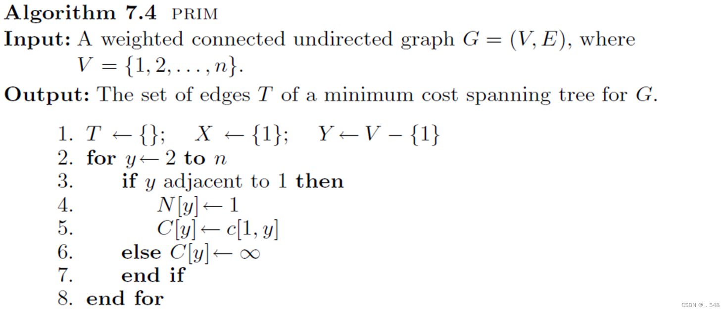
Minimum Cost Spanning Trees (Prim’s Algorithm)
(1) T ←{}; X ←{1}; Y ←V − {1}
(2) while Y = {}
(3) Let (x, y) be of minimum weight such that x ∈ X and y ∈ Y .
(4) X←X ∪ {y}
(5) Y ←Y −{y}
(6) T←T ∪ {(x, y)}
(7) end while
Example 7.4 Consider the graph shown in Fig. 7.5(a). The vertices to the left of the dashed line belong to X, and those to its right belong to Y . First, as shown in Fig. 7.5(a), X = {1} and Y = {2, 3, . . . , 6}. In Fig. 7.5(b), vertex 2 is moved from Y to X since edge (1, 2) has the least cost among all the edges incident to vertex 1. This is indicated by moving the dashed line so that 1 and 2 are now to its left.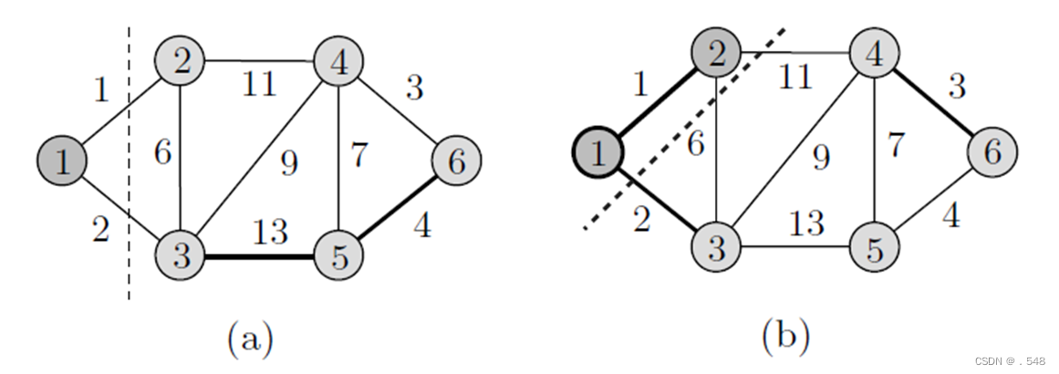 As shown in Fig. 7.5(b), the candidate vertices to be moved from Y to X are 3 and 4. Since edge (1, 3) is of least cost among all edges with one end in X and one end in Y , 3 is moved from Y to X. Next, from the two candidate vertices 4 and 5 in Fig. 7.5(c), 4 is moved since the edge (3, 4) has the least cost.
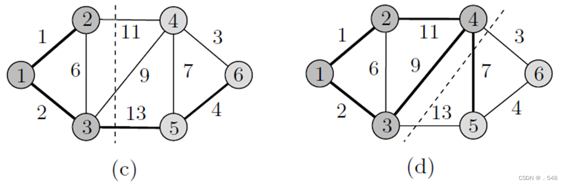 Finally, vertices 6 and then 5 are moved from Y to X as shown in Fig. 7.5(e). Each time a vertex y is moved from Y to X, its corresponding edge is included in T , the set of edges of the minimum spanning tree. The resulting minimum spanning tree is shown in Fig. 7.5(f).
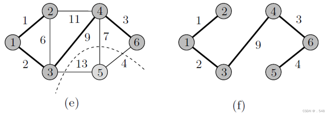
 Time complexity: Θ(n**2)Theorem 7.4 Algorithm PRIM finds a minimum cost spanning tree in a weighted undirected graph with n vertices in Θ(n**2) time.
Lemma 7.3 Algorithm PRIM correctly finds a minimum cost spanning tree in a connected undirected graph.
File Compression
Let F be a characters stream file, where the characters are taken from the set C ={c1, c2,…, cn}. Let also f(ci), 1 ≤ i ≤ n, be the frequency of character ci in the file, i.e., the number of times ci appears in the file. We hope to compress the file in a way that is as small as possible and easy to recover from the compressed file.
Using a fixed length number of bits to represent, called the fixed-length encoding.
Using variable-length encodings. Intuitively, those characters with large frequencies should be assigned short encodings.
When the encodings vary in length, we stipulate that the encoding of one character must not be the prefix of the encoding of another character; such codes are called prefix codes. For instance, if we assign the encodings 10 and 101 to the letters “a” and “b”, there will be an ambiguity as to whether 10 is the encoding of “a” or is the prefix of the encoding of the letter “b”.
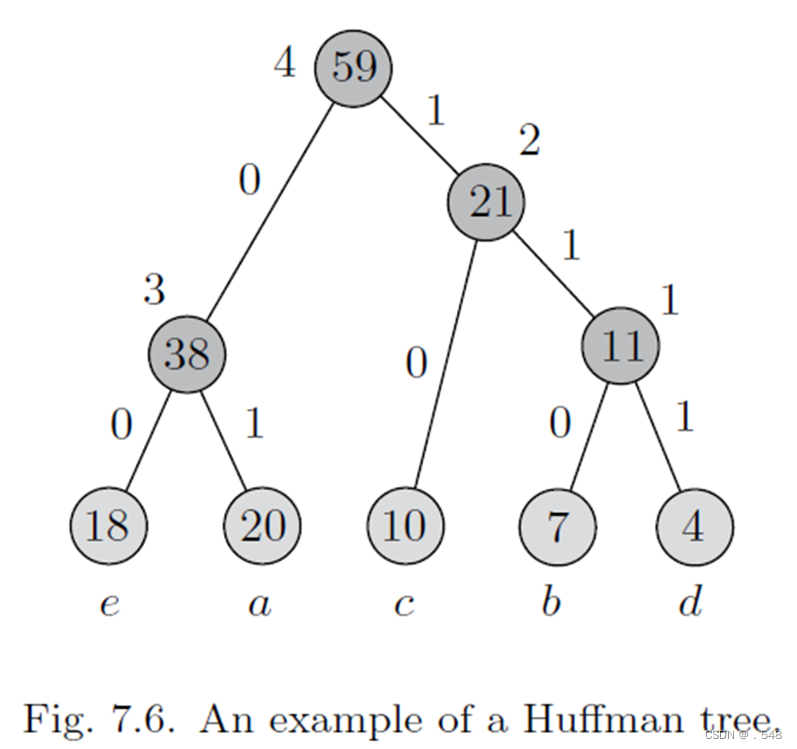
Example 7.5 Consider finding a prefix code for a file that consists of the letters a, b, c, d, and e. Suppose that these letters appear in the file with the following frequencies: f(a) = 20, f(b) = 7, f(c) = 10, f(d) = 4 and f(e) = 18.
Each leaf node is labeled with its corresponding character and its frequency of occurrence in the file. Each internal node is labeled with the sum of the weights of the leaves in its subtree and the order of its creation. For instance, the first internal node created has a sum of 11 and it is labeled with 1. From the binary tree, the encodings for a, b, c, d, and e are, respectively, 01, 110, 10, 111, and 00. Suppose each character was represented by three binary digits before compression. Then, the original size of the file is 3(20+7+10+4+18) = 177 bits. The size of the compressed file using the above code becomes 2 × 20 + 3 × 7 + 2 × 10 + 3 × 4 + 2 × 18 = 129 bits, a saving of about 27%. See Fig. 7.6.