Machine Learning - Logistic Regression

目录

一、Activation Function

Why introduce activation functions?

There are several commonly used activation functions:

二、Sigmoid：

三、Logistic Regression Model：

四、Implementation of logistic regression：

五、Decision Boundary：

一、Activation Function

        In logistic regression, the function of the activation function is to convert the output of the linear model into a probability value, so that it can represent the probability that the sample belongs to a certain category. Logistic regression is a binary classification algorithm that calculates the linear combination of input features and maps the results through an activation function to obtain a probability value between 0 and 1.

Why introduce activation functions?

        ①Converting the output of a linear model into probability values: The goal of logistic regression is to predict the probability that a sample belongs to a certain category, while the output of a linear model is a continuous real number value. By activating the function, the output of the linear model can be mapped between 0 and 1, representing the probability that the sample belongs to a certain category.
        ② Introducing non-linear relationships: The activation function introduces non-linear relationships, enabling the logistic regression model to fit non-linear data. If there is no activation function, logistic regression becomes linear regression and cannot handle non-linear classification problems.
        ③ The need for gradient calculation: The derivative of the activation function plays an important role in gradient descent algorithms. By activating the derivative of the function, the gradient of model parameters can be calculated, thereby optimizing and updating the model.

There are several commonly used activation functions:

        Sigmoid、Tanh Function、ReLU Function（Rectified Linear Unit）、Leaky ReLU、ELU Function（Exponential Linear Unit）、Softmax Function.

二、Sigmoid：

        The sigmoid function is one of the commonly used activation functions in logistic regression, which has the following characteristics that make it suitable for use in logistic regression.
        ① The output can be mapped to a probability value between 0 and 1: the output range of the sigmoid function is between 0 and 1, and the result of linear combination can be transformed into a probability value, representing the probability that the sample belongs to a certain category. This meets the classification task requirements of logistic regression.
        ② Differentiability: The sigmoid function is differentiable throughout the entire domain, which is crucial for parameter updates using optimization algorithms such as gradient descent. By taking the derivative, the gradient of the loss function on the parameters can be obtained, thereby updating the model parameters.
        ③ Having monotonicity: The sigmoid function is a monotonically increasing function, which means that as the input increases, the output also increases. This is helpful for learning and optimizing the model.
        ④ Smoothness: The sigmoid function is smooth throughout the entire domain, without any abrupt or discontinuous points. This helps to improve the stability and convergence of the model.

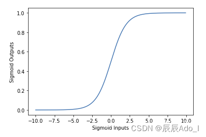
The complete formula is:

The image is as follows:

三、Logistic Regression Model：

        Logistic regression is a linear classifier (linear model) primarily used for binary classification problems. There are only two types of classification results: 1 and 0.

四、Implementation of logistic regression：

        Assuming that we determine whether a tumor is malignant or benign based on its size, we assume the following dataset:

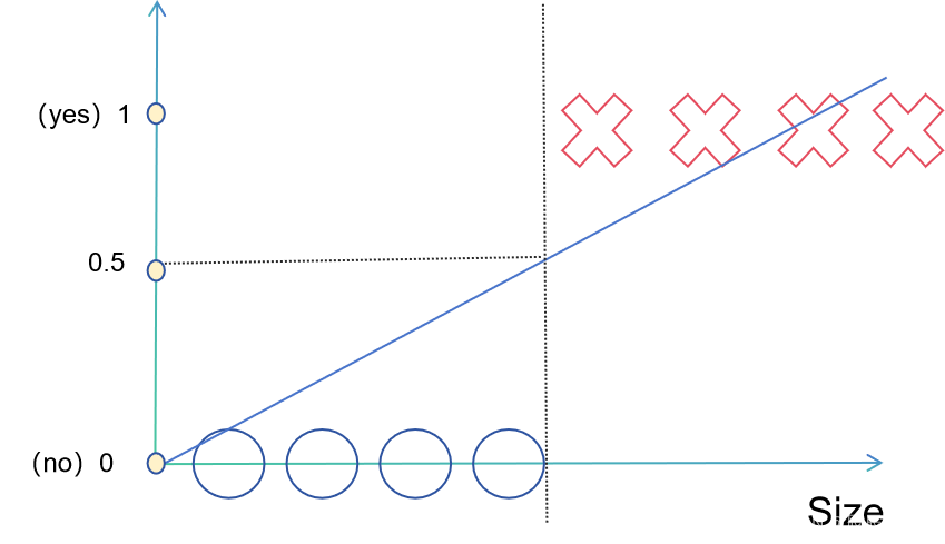
        We assume that 1 corresponds to malignancy and 0 corresponds to benign. Then, based on linear regression, we draw a straight line in the graph, and we divide it by the midpoint 0.5 of the interval [0,1] corresponding to the y-axis.

        We can assume that when the value of the corresponding equation  is greater than 0.5, the corresponding tumor is benign, otherwise it is malignant. This is a situation where the dataset is relatively balanced. What if there is an outlier?

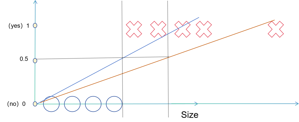
        Obviously, the results have become less reasonable, so using only linear regression to perform logistic regression is not feasible. At this point, we need to use the commonly used activation function in logistic regression:
        Firstly, we want to fix the result of y between 0 and 1, so that it is easier to determine whether the value is 0 or 1 when making discrete value predictions. So at this point, choose a function, which is the sigmoid function, which is an S-type function with a value range of (0,1), and can map a real number to the interval of (0,1), which exactly meets all the requirements.
        We can obtain the following equation by incorporating our linear regression function into the sigmoid function:

        Now, we can make predictions using the above equation. Next, we will further understand what decision boundaries are.

五、Decision Boundary：

        The decision boundary of logistic regression is a hyperplane, which divides the feature space into two regions corresponding to different categories. In binary classification problems, the decision boundary can be viewed as a straight line or curve, dividing the feature space into positive and negative classes. In multi classification problems, the decision boundary can be a hyperplane or a combination of multiple hyperplanes.
        The position of the decision boundary depends on the parameters of the logistic regression model. The logistic regression model determines the optimal decision boundary by learning the relationship between features and labels in the training data. The model optimizes parameters by maximizing the likelihood function or minimizing the loss function, in order to find the optimal decision boundary.
        After using the sigmoid function, we can specify the output rules for its results as follows:

        So we can easily find the corresponding linear regression equation:

        The straight line corresponding to its z is what we call the decision boundary:

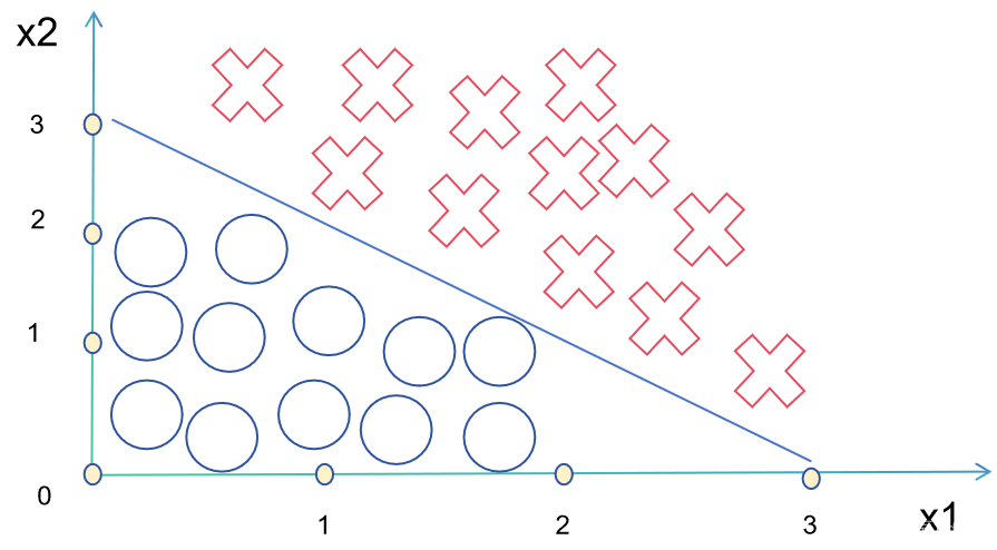
        Of course, not all decision boundaries are linear, and there are also many nonlinear decision boundaries. We can change the shape of the decision boundaries by adding polynomials.